Page 288 - Soil and water contamination, 2nd edition

Model calibration and validation 275

-4
x 10
1.8
6642 6642 6642
1.7 0.011
1.6 0.010
1.5
1.4
-1
2 s (m .s ) 1.3
q 0.009
1.2
1.1 0.011 0.010
1.0 0.014 0.013 0.012
0.9 0.016 0.015
0.8
0.50 0.60 0.70 0.80 0.90
-1
k (day )
p
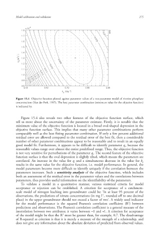
Figure 15.4 Objective function plotted against parameter values of a two-parameter model of riverine phosphate
concentrations (Van der Perk, 1997). The best parameter combination (minimum value for the objective function)
is indicated by.

Figure 15.4 also reveals two other features of the objective function surface, which
tell us more about the uncertainty of the parameter estimate. Firstly, it is notable that the
minimum value of the objective function is located in a broad oval-shaped depression in the
objective function surface. This implies that many other parameter combinations perform
comparably well as the best fitting parameter combination. If only a few percent additional
residual error are allowed compared to the residual error of the best fit, then a considerable
number of other parameter combinations appear to be reasonable and to result in an equally
good model fit. Furthermore, it appears to be difficult to identify parameter q , because the
s
reasonable values range over almost the entire predefined range. Thus, the objective function
is not very sensitive for perturbations of the parameter q . The second feature of the objective
s
function surface is that the oval depression is slightly tilted, which means the parameters are
correlated. An increase in the value for q and a simultaneous decrease in the value for k
s p
results in the same value for the objective function, i.e. model performance. In general, the
model parameters become more difficult to identify uniquely if the correlation between the
parameters increases. Such a sensitivity analysis of the objective function, which includes
both an assessment of the residual error in the parameter values and the correlations between
parameters, thus provides useful information on the identifiability of the parameters.
To validate a model in a quantitative manner, various statistical criteria for model
acceptance or rejection can be established. A criterion for acceptance of a catchment-
scale model of nitrogen leaching into groundwater could be: ‘In at least 95 percent of the
-1
observations, the predictions of nitrate concentrations (in mg l , rounded off to one decimal
place) in the upper groundwater should not exceed a factor of two’. A widely used indicator
2
for the model performance is the squared Pearson’s correlation coefficient (R ) between
predictions and observations. The Pearson’s correlation coefficient is a general measure of the
interrelation between two attributes; it varies between –1 and +1. A criterion for acceptance
2
of the model might be that the R must be greater than, for example, 0.7. The disadvantage
of R-squared as criterion is that it is merely a measure of the strength of a relationship, and
does not give any information about the absolute deviation of predicted from observed values.

10/1/2013 6:45:22 PM
Soil and Water.indd 287 10/1/2013 6:45:22 PM
Soil and Water.indd 287