Page 291 - Soil and water contamination, 2nd edition

278 Soil and Water Contamination

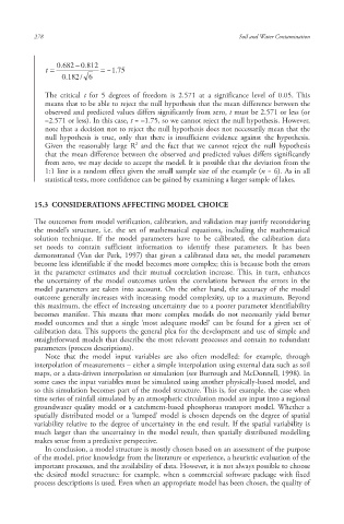
. 0 682 . 0 812
t . 1 75
. 0 182 / 6

The critical t for 5 degrees of freedom is 2.571 at a significance level of 0.05. This
means that to be able to reject the null hypothesis that the mean difference between the
observed and predicted values differs significantly from zero, t must be 2.571 or less (or
–2.571 or less). In this case, t = –1.75, so we cannot reject the null hypothesis. However,
note that a decision not to reject the null hypothesis does not necessarily mean that the
null hypothesis is true, only that there is insufficient evidence against the hypothesis.
2
Given the reasonably large R and the fact that we cannot reject the null hypothesis
that the mean difference between the observed and predicted values differs significantly
from zero, we may decide to accept the model. It is possible that the deviation from the
1:1 line is a random effect given the small sample size of the example (n = 6). As in all
statistical tests, more confidence can be gained by examining a larger sample of lakes.

15.3 CONSIDERATIONS AFFECTING MODEL CHOICE

The outcomes from model verification , calibration , and validation may justify reconsidering
the model’s structure, i.e. the set of mathematical equations, including the mathematical
solution technique. If the model parameters have to be calibrated, the calibration data
set needs to contain sufficient information to identify these parameters. It has been
demonstrated (Van der Perk, 1997) that given a calibrated data set, the model parameters
become less identifiable if the model becomes more complex; this is because both the errors
in the parameter estimates and their mutual correlation increase. This, in turn, enhances
the uncertainty of the model outcomes unless the correlations between the errors in the
model parameters are taken into account. On the other hand, the accuracy of the model
outcome generally increases with increasing model complexity, up to a maximum. Beyond
this maximum, the effect of increasing uncertainty due to a poorer parameter identifiability
becomes manifest. This means that more complex models do not necessarily yield better
model outcomes and that a single ‘most adequate model’ can be found for a given set of
calibration data. This supports the general plea for the development and use of simple and
straightforward models that describe the most relevant processes and contain no redundant
parameters (process descriptions).
Note that the model input variables are also often modelled: for example, through
interpolation of measurements – either a simple interpolation using external data such as soil
maps, or a data-driven interpolation or simulation (see Burrough and McDonnell, 1998). In
some cases the input variables must be simulated using another physically-based model, and
so this simulation becomes part of the model structure. This is, for example, the case when
time series of rainfall simulated by an atmospheric circulation model are input into a regional
groundwater quality model or a catchment-based phosphorus transport model. Whether a
spatially distributed model or a ‘lumped’ model is chosen depends on the degree of spatial
variability relative to the degree of uncertainty in the end result. If the spatial variability is
much larger than the uncertainty in the model result, then spatially distributed modelling
makes sense from a predictive perspective.
In conclusion, a model structure is mostly chosen based on an assessment of the purpose
of the model, prior knowledge from the literature or experience, a heuristic evaluation of the
important processes, and the availability of data. However, it is not always possible to choose
the desired model structure: for example, when a commercial software package with fixed
process descriptions is used. Even when an appropriate model has been chosen, the quality of

10/1/2013 6:45:23 PM
Soil and Water.indd 290 10/1/2013 6:45:23 PM
Soil and Water.indd 290