Page 287 - Soil and water contamination, 2nd edition

274 Soil and Water Contamination

To obtain optimal and reproducible calibrated parameter values, a more quantitative
approach is preferable. Such an approach requires the model performance criteria to be
quantified, formalised in an objective function . In mathematical terms, this objective
function describes the difference between observed values and model predictions, given
a set of model parameter values; these differences could be the absolute differences or the
squared differences, for example. The outcome of the objective function thus varies with
varying values for the model parameter values. The calibration procedure aims at finding
the minimum of this function; once this has been done, the associated parameter values are
considered to be the best estimates. Often, the sum of the square of the differences between
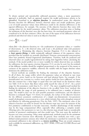
predicted and observed values is used as an objective function:
n
ˆ
) f ( ~ i x ( q) x 2 (15.1)
i
i 1
where f(α) = the objective function , α = the combination of parameter values, n = number
~
of observations, x = ith observed value, and ˆ x i (q ) = ith predicted value with parameter
i
combination q. Minimising this objective function (Equation 15.1) is also referred to
as least squares fitting ; it yields statistically unbiased estimates of the parameter values,
provided that the residuals are normally distributed. However, environmental concentrations
often have positively skewed (lognormal) distributions. Therefore, both the predicted and
observed values are usually logtransformed by taking their logarithm before calculating the
residuals. If the model predicts two or more variables for which observed data are available
for calibration , the least squares criterion (Equation 15.1) can also be used, but the residuals
of the different variables should be weighted proportional to the reciprocal of the means or
variances of the respective variables, otherwise the variable with the largest absolute values
dominates the calibration result.
Several methods are available for finding the minimum of the objective function .
In all of them, the ranges within which the parameter values are allowed to vary must
be defined a priori, based on the literature and hard physical limits. For example, if the
denitrification rate constant in a surface water quality model has been calibrated, we know
that this constant has a value larger or equal than zero and based on the literature values
-1
(see Table 13.3) we know that these values rarely exceed the value of 2.0 d . An a priori
-1
range for this parameter could thus be 0 – 2.0 d . The most straightforward method for
finding the minimum of the objective function is the so-called ‘brute force’ method: this
method divides the range of each parameter to be calibrated into a number of discrete
steps. The model is then run for each possible parameter combination, and the objective
function is evaluated. Figure 15.4 shows, for example, the surface of the objective function
for the different parameter combinations of a simple one-dimensional, two-parameter
model of phosphate concentrations in a river, which includes first-order phosphate removal
and dilution by inflowing groundwater (Van der Perk, 1997). The minimum value of the
objective function can easily be found, but the discrete steps may cause the estimate of the
best parameter combination to become inaccurate. Another disadvantage of this method
may be the large computational effort, especially when calibrating a complex model.
Allowing only a few parameters to vary in a few discrete steps already leads to considerable
number of parameter combinations and thus model runs. This may cause the method to
become very time-consuming. Other, more sophisticated, methods search for the minimum
of the objective function more efficiently. In general, these methods start with a user-
defined initial parameter estimate after which the minimum is searched for iteratively. This
automated calibration is also referred to as inverse modelling . There are several computer
tools available for automated calibration, e.g. PEST (WHI, 1999) and UCODE (Poeter and
Hill, 1998).

10/1/2013 6:45:21 PM
Soil and Water.indd 286 10/1/2013 6:45:21 PM
Soil and Water.indd 286