Page 136 - Statistics II for Dummies

120 Part II: Using Different Types of Regression to Make Predictions

polynomial. The general form for a polynomial regression model is
1
2
k
3
y = β + β x + β x + β x + . . . + β x + ε. Here, k represents the total number of
0 1 2 3 k
terms in the model. The ε represents the error that occurs simply due to chance.
(Not a bad kind of error, just random fluctuations from a perfect model.)
Here are a few of the more common polynomials you run across when ana-
lyzing data and fitting models. Remember, the simplest model that fits is the
one you use (don’t try to be a hero in statistics — save that for Batman and
Robin). The models I discuss in this book are some of your old favorites from
algebra: second-, third-, and fourth-degree polynomials.
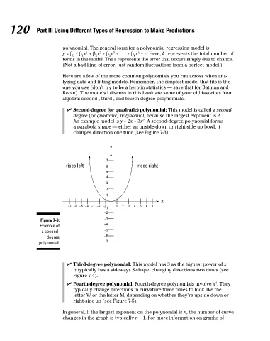
✓ Second-degree (or quadratic) polynomial: This model is called a second-
degree (or quadratic) polynomial, because the largest exponent is 2.
2
An example model is y = 2x + 3x . A second-degree polynomial forms
a parabola shape — either an upside-down or right-side up bowl; it
changes direction one time (see Figure 7-3).

y

7
rises left 6 rises right
5
4
3
2
1
x
−7 −6 −5 −4 −3 −2 −1 1 2 3 4 5 6 7
−1
−2
Figure 7-3: −3
Example of −4
a second- −5
degree −6
polynomial. −7

✓ Third-degree polynomial: This model has 3 as the highest power of x.
It typically has a sideways S-shape, changing directions two times (see
Figure 7-4).
4
✓ Fourth-degree polynomial: Fourth-degree polynomials involve x . They
typically change directions in curvature three times to look like the
letter W or the letter M, depending on whether they’re upside down or
right-side up (see Figure 7-5).

In general, if the largest exponent on the polynomial is n, the number of curve
changes in the graph is typically n – 1. For more information on graphs of

12_466469-ch07.indd 120 7/24/09 9:39:08 AM