Page 156 - Statistics II for Dummies

140
Part II: Using Different Types of Regression to Make Predictions
If you were to estimate p using a simple linear regression model, you may
think you should try to fit a straight line, p = β + β x. However, it doesn’t
0 1
make sense to use a straight line to estimate the probability of an event
occurring based on another variable, due to the following reasons:
✓ The estimated values of p can never be outside of [0, 1], which goes
against the idea of a straight line (a straight line continues on in both
directions).
✓ It doesn’t make sense to force the values of p to increase in a linear
way based on x. For example, an event may occur very frequently with
a range of large values of x and very frequently with a range of small
values of x, with very little chance of the event happening in an area
in between. This type of model would have a U shape rather than a
straight-line shape.

To come up with a more appropriate model for p, statisticians created a new
function of p whose graph is called an S-curve. The S-curve is a function that
involves p, but it also involves e (the natural logarithm) as well as a ratio of
two functions.

The values of the S-curve always fit between 0 and 1, which allows the prob-
ability, p, to change from low to high or high to low, according to a curve
that’s shaped like an S. The general form of the logistic regression model
based on an S-curve is .

Interpreting the coefficients of

the logistic regression model

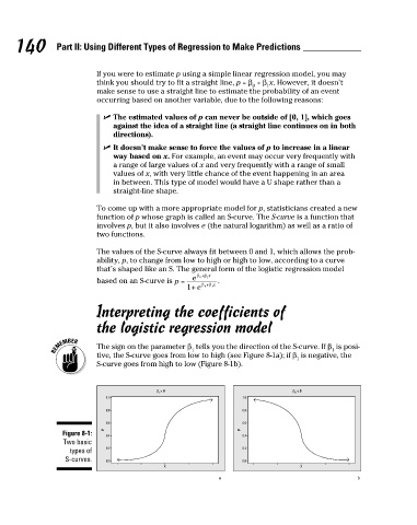
The sign on the parameter β tells you the direction of the S-curve. If β is posi-
1 1
tive, the S-curve goes from low to high (see Figure 8-1a); if β is negative, the
1
S-curve goes from high to low (Figure 8-1b).

β 1 > 0 β 1 < 0
1.0 1.0
0.8 0.8
0.6 0.6
p p
Figure 8-1: 0.4 0.4
Two basic
types of 0.2 0.2
S-curves. 0.0 0.0
X X
a b

7/23/09 9:28:36 PM
13_466469-ch08.indd 140 7/23/09 9:28:36 PM
13_466469-ch08.indd 140