Page 171 - Statistics II for Dummies

Chapter 9: Testing Lots of Means? Come On Over to ANOVA!
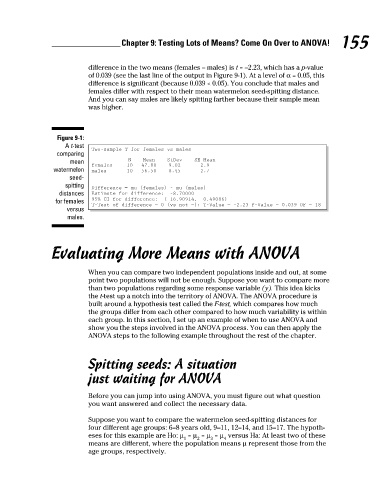
difference in the two means (females – males) is t = –2.23, which has a p-value 155
of 0.039 (see the last line of the output in Figure 9-1). At a level of α = 0.05, this
difference is significant (because 0.039 < 0.05). You conclude that males and
females differ with respect to their mean watermelon seed-spitting distance.
And you can say males are likely spitting farther because their sample mean
was higher.

Figure 9-1:
A t-test
Two-sample T for females vs males
comparing
mean N Mean StDev SE Mean
females 10 47.80 9.02 2.9
watermelon males 10 56.50 8.45 2.7
seed-
spitting
Difference = mu (females) – mu (males)
distances Estimate for difference: –8.70000
for females 95% CI for difference: (–16.90914, –0.49086)
T–Test of difference = 0 (vs not =): T–Value = –2.23 P–Value = 0.039 DF = 18
versus
males.

Evaluating More Means with ANOVA

When you can compare two independent populations inside and out, at some
point two populations will not be enough. Suppose you want to compare more
than two populations regarding some response variable (y). This idea kicks
the t-test up a notch into the territory of ANOVA. The ANOVA procedure is
built around a hypothesis test called the F-test, which compares how much
the groups differ from each other compared to how much variability is within
each group. In this section, I set up an example of when to use ANOVA and
show you the steps involved in the ANOVA process. You can then apply the
ANOVA steps to the following example throughout the rest of the chapter.

Spitting seeds: A situation

just waiting for ANOVA

Before you can jump into using ANOVA, you must figure out what question
you want answered and collect the necessary data.
Suppose you want to compare the watermelon seed-spitting distances for
four different age groups: 6–8 years old, 9–11, 12–14, and 15–17. The hypoth-
eses for this example are Ho: μ = μ = μ = μ versus Ha: At least two of these
1 2 3 4
means are different, where the population means μ represent those from the
age groups, respectively.

7/23/09 9:31:28 PM
15_466469-ch09.indd 155
15_466469-ch09.indd 155 7/23/09 9:31:28 PM