Page 181 - Statistics II for Dummies

Chapter 9: Testing Lots of Means? Come On Over to ANOVA!
The Minitab output for the watermelon seed-spitting contest for the four age 165
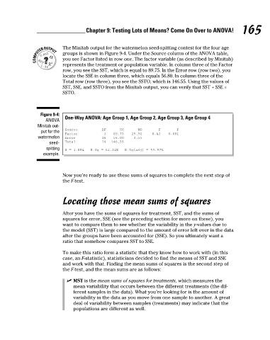
groups is shown in Figure 9-4. Under the Source column of the ANOVA table,
you see Factor listed in row one. The factor variable (as described by Minitab)
represents the treatment or population variable. In column three of the Factor
row, you see the SST, which is equal to 89.75. In the Error row (row two), you
locate the SSE in column three, which equals 56.80. In column three of the
Total row (row three), you see the SSTO, which is 146.55. Using the values of
SST, SSE, and SSTO from the Minitab output, you can verify that SST + SSE =
SSTO.

Figure 9-4:
One-Way ANOVA: Age Group 1, Age Group 2, Age Group 3, Age Group 4
ANOVA
Minitab out-
Source DF SS MS F P
put for the
Factor 3 89.75 29.92 8.43 0.001
watermelon Error 16 56.80 3.55
seed- Total 19 146.55
spitting
S = 1.884 R–Sq = 61.24% R–Sq(adj) = 53.97%
example.

Now you’re ready to use these sums of squares to complete the next step of
the F-test.

Locating those mean sums of squares

After you have the sums of squares for treatment, SST, and the sums of
squares for error, SSE (see the preceding section for more on these), you
want to compare them to see whether the variability in the y-values due to
the model (SST) is large compared to the amount of error left over in the data
after the groups have been accounted for (SSE). So you ultimately want a
ratio that somehow compares SST to SSE.

To make this ratio form a statistic that they know how to work with (in this
case, an F-statistic), statisticians decided to find the means of SST and SSE
and work with that. Finding the mean sums of squares is the second step of
the F-test, and the mean sums are as follows:
✓ MST is the mean sums of squares for treatments, which measures the
mean variability that occurs between the different treatments (the dif-
ferent samples in the data). What you’re looking for is the amount of
variability in the data as you move from one sample to another. A great
deal of variability between samples (treatments) may indicate that the
populations are different as well.

7/23/09 9:31:30 PM
15_466469-ch09.indd 165 7/23/09 9:31:30 PM
15_466469-ch09.indd 165