Page 284 - Statistics II for Dummies

268 Part IV: Building Strong Connections with Chi-Square Tests

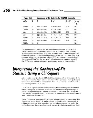
Table 15-3 Goodness-of-Fit Statistic for M&M’S Example
Color O E O – E (O – E) 2

Brown 4 0.13 * 56 = 7.28 4 – 7.28 = –3.28 10.76 1.48
Yellow 10 0.14 * 56 = 7.84 10 – 7.84 = 2.16 4.67 0.60
Red 4 0.13 * 56 = 7.28 4 – 7.28 = –3.28 10.76 1.48
Blue 10 0.24 * 56 = 13.44 10 – 13.44 = –3.44 11.83 0.88
Orange 15 0.20 * 56 = 11.20 15 – 11.20 = 3.80 14.44 1.29
Green 13 0.16 * 56 = 8.96 13 – 8.96 = 4.04 16.32 1.82
TOTAL 56 56 7.55

The goodness-of-fit statistic for the M&M’S example turns out to be 7.55,
the bolded number in the lower-right corner of Table 15-3. This number
represents the total squared difference between what I expected and what I
observed, adjusted for the magnitude of each expected cell count. The next
question is how to interpret this value of 7.55. Is it large enough to indicate
that colors of M&M’S in the bag aren’t following the percentages posted by
Mars? The next section addresses how to make sense of these results.

Interpreting the Goodness-of-Fit

Statistic Using a Chi-Square

After you get your goodness-of-fit statistic, your next job is to interpret it. To
do this, you need to figure out the possible values you could have gotten and
where your statistic fits in among them. You can accomplish this task with a
Chi-square goodness-of-fit test.

The values of a goodness-of-fit statistic actually follow a Chi-square distribution
with k – 1 degrees of freedom, where k is the number of categories in your
particular population (see Chapter 14 for the full details on the Chi-square).
You use the Chi-square table (Table A-3 in the appendix) to find the p-value of
your Chi-square test statistic.

If your Chi-square goodness-of-fit statistic is large enough, you conclude that
the original model doesn’t fit and you have to chuck it; there’s too much of
a difference between what you observed and what you expected under the
model. However, if your goodness-of-fit statistic is relatively small, you don’t

22_466469-ch15.indd 268 7/24/09 9:52:21 AM