Page 176 - Statistics and Data Analysis in Geology

Analysis of Multivariate Data

3. Mutual similarity procedures group together observations that have a common
similarity to other observations. First an n x n matrix of similarities between
all pairs of observations is calculated. Then the similarity between columns
of this matrix is iteratively recomputed. Columns representing members of a
single cluster will tend to have intercorrelations near +1, while having much
lower correlations with nonmembers.
4. Hierarchical clustering joins the most similar observations, then successively
connects the next most similar observations to these. First an n x n matrix of
similarities between all pairs of observations is calculated. Those pairs having
the highest similarities are then merged, and the matrix is recomputed. This
is done by averaging the similarities that the combined observations have with
other observations. The process iterates until the similarity matrix is reduced
to 2 x 2. The progression of levels of similarity at which observations merge is
displayed as a dendrogram.
Hierarchical clustering techniques are most widely applied in the Earth sci-
ences, probably because their development has been closely linked with the numer-
ical taxonomy of fossil organisms. Because of the widespread use of heirarchical
techniques, we will consider them in some detail.
Suppose we have a collection of objects we wish to arrange into a hierarchical
classification. In biology, these objects are referred to as “operational taxonomic
units” or OW’S (Sneath and Sokal, 1973). We can make a series of measurements
on each object which constitutes our data set. If we have n objects and measure m
characteristics, the observations form an nx m data matrix, X. Next, some measure
of resemblance or similarity must be computed between every pair of objects; that
is, between the rows of the data matrix. Several coefficients of resemblance have
been used, including a variation of the correlation coefficient fij in which the roles
of objects and variables are interchanged. This can be done by transposing X so
rows become columns and vice versa, then calculating fij in the conventional man-
ner (Eq. 2.28; p. 43), following the matrix algorithm given in Chapter 3. Although
called “correlation,” this measure is not really a correlation coefficient in the con-
ventional sense because it involves “means” and “variances” calculated across all
the variables measured on two objects, rather than the means and variances of two
variables.
Another commonly used measure of similarity between objects is a standard-
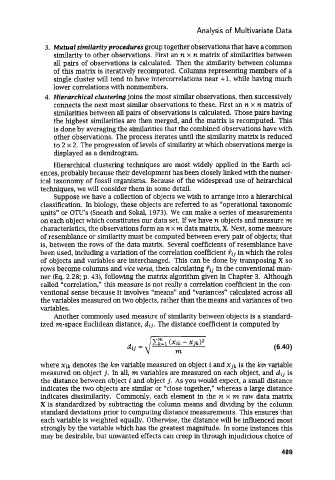
ized m-space Euclidean distance, dij. The distance coefficient is computed by

(6.40)

where Xik denotes the kth variable measured on object i and xjk is the kth variable
measured on object j. In all, m variables are measured on each object, and dij is
the distance between object i and object j. As you would expect, a small distance
indicates the two objects are similar or “close together,” whereas a large distance
indicates dissimilarity. Commonly, each element in the n x m raw data matrix
X is standardized by subtracting the column means and dividing by the column
standard deviations prior to computing distance measurements. This ensures that
each variable is weighted equally. Otherwise, the distance will be influenced most
strongly by the variable which has the greatest magnitude. In some instances this
may be desirable, but unwanted effects can creep in through injudicious choice of

489