Page 178 - Statistics and Data Analysis in Geology

Analysis of Multivariate Data

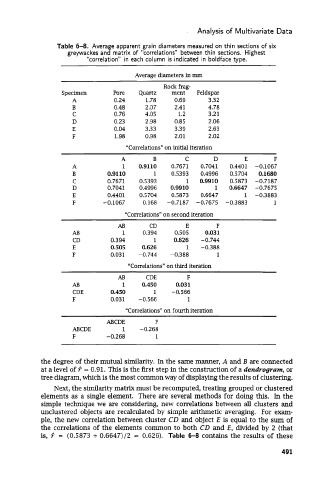
Table 6-8. Average apparent grain diameters measured on thin sections of six
greywackes and matrix of “correlations” between thin sections. Highest
“correlation” in each column is indicated in boldface type.

Average diameters in mm

Rock frag-
Specimen Pore Quartz ment Feldspar
A 0.24 1.78 0.69 3.32
B 0.48 2.07 2.41 4.78
C 0.76 4.05 1.2 3.21
D 0.23 2.98 0.85 2.06
E 0.04 3.33 3.39 2.63
F 1.98 0.98 2.01 2.02
“Correlations” on initial iteration
A B C D E F
A 1 0,9110 0.7671 0.7041 0.4401 -0.1067
B 0.91 10 1 0.5393 0.4996 0.5704 0.1680
C 0.7671 0.5393 1 0.9910 0.5873 -0.7187
D 0.7041 0.4996 0.9910 1 0.6647 -0.7675
E 0.4401 0.5704 0.5873 0.6647 1 -0.3883
F -0.1067 0.168 -0.7187 -0.7675 -0.3883 1

“Correlations” on second iteration
AB CD E F
AB 1 0.394 0.505 0.031
CD 0.394 1 0.626 -0.744
E 0.505 0.626 1 -0.388
F 0.031 -0.744 -0.388 1
“Correlations” on third iteration
AB CDE F
AB 1 0.450 0.031
CDE 0.450 1 -0.566
F 0.031 -0.566 1
“Correlations” on fourth iteration
ABCDE F
ABCDE 1 -0.268
F -0.268 1

the degree of their mutual similarity. In the same manner, A and B are connected
at a level of Q = 0.91. This is the first step in the construction of a dendrogrum, or
tree diagram, which is the most common way of displaying the results of clustering.
Next, the similarity matrix must be recomputed, treating grouped or clustered
elements as a single element. There are several methods for doing this. In the
simple technique we are considering, new correlations between all clusters and
unclustered objects are recalculated by simple arithmetic averaging. For exam-
ple, the new correlation between cluster CD and object E is equal to the sum of
the correlations of the elements collZmon to both CD and E, divided by 2 (that
is, Q = (0.5873 + 0.6647)/2 = 0.626). Table 6-8 contains the results of these

491