Page 104 - Statistics for Environmental Engineers

L1592_Frame_C11 Page 99 Tuesday, December 18, 2001 1:47 PM

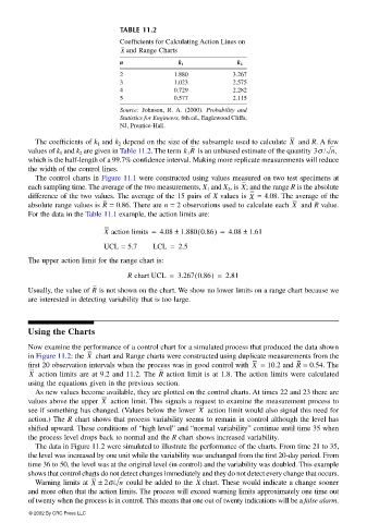
TABLE 11.2
Coefficients for Calculating Action Lines on
X and Range Charts
n k 1 k 2
2 1.880 3.267
3 1.023 2.575
4 0.729 2.282
5 0.577 2.115
Source: Johnson, R. A. (2000). Probability and
Statistics for Engineers, 6th ed., Englewood Cliffs,
NJ, Prentice-Hall.
The coefficients of k 1 and k 2 depend on the size of the subsample used to calculate X and R. A few
values of k 1 and k 2 are given in Table 11.2. The term k 1 R is an unbiased estimate of the quantity 3σ / n,
which is the half-length of a 99.7% confidence interval. Making more replicate measurements will reduce
the width of the control lines.
The control charts in Figure 11.1 were constructed using values measured on two test specimens at
each sampling time. The average of the two measurements, X 1 and X 2 , is ; and the range R is the absoluteX
difference of the two values. The average of the 15 pairs of X values is = 4.08. The average of the
X
absolute range values is = 0.86. There are n = 2 observations used to calculate eachR X and R value.
For the data in the Table 11.1 example, the action limits are:
(
X action limits = 4.08 ± 1.880 0.86) = 4.08 ± 1.61
UCL = 5.7 LCL = 2.5

The upper action limit for the range chart is:
(
R chart UCL = 3.267 0.86) = 2.81
R
Usually, the value of is not shown on the chart. We show no lower limits on a range chart because we
are interested in detecting variability that is too large.

Using the Charts

Now examine the performance of a control chart for a simulated process that produced the data shown
in Figure 11.2: the X chart and Range charts were constructed using duplicate measurements from the
R
first 20 observation intervals when the process was in good control with X = 10.2 and = 0.54. The
R
X action limits are at 9.2 and 11.2. The action limit is at 1.8. The action limits were calculated
using the equations given in the previous section.
As new values become available, they are plotted on the control charts. At times 22 and 23 there are
values above the upper X action limit. This signals a request to examine the measurement process to
see if something has changed. (Values below the lower X action limit would also signal this need for
action.) The R chart shows that process variability seems to remain in control although the level has
shifted upward. These conditions of “high level” and “normal variability” continue until time 35 when
the process level drops back to normal and the R chart shows increased variability.
The data in Figure 11.2 were simulated to illustrate the performance of the charts. From time 21 to 35,
the level was increased by one unit while the variability was unchanged from the first 20-day period. From
time 36 to 50, the level was at the original level (in control) and the variability was doubled. This example
shows that control charts do not detect changes immediately and they do not detect every change that occurs.
Warning limits at X ± 2σ/ n could be added to the X chart. These would indicate a change sooner
and more often that the action limits. The process will exceed warning limits approximately one time out
of twenty when the process is in control. This means that one out of twenty indications will be a false alarm.
© 2002 By CRC Press LLC