Page 147 - Statistics for Environmental Engineers

L1592_Frame_C16 Page 144 Tuesday, December 18, 2001 1:51 PM

a

t = 2.35
0

3 2 1 0 1 2 3
y — η
t statistic, t =
s
y
b
y — η = 0.2
0

- 0.3 - 0.2 - 0.1 0 0.1 0.2 0.3
True difference, y — η – s t
y
c

η = 1.2
0

1.1 1.2 1.3 1.4 1.5 1.6 1.7
True mean, η = y – s t
y

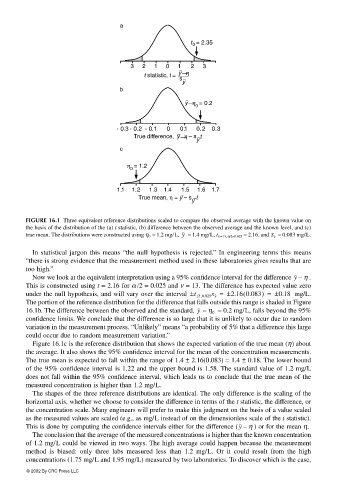
FIGURE 16.1 Three equivalent reference distributions scaled to compare the observed average with the known value on
the basis of the distribution of the (a) t statistic, (b) difference between the observed average and the known level, and (c)
y = 0.083 mg/L.
true mean. The distributions were constructed using η 0 = 1.2 mg/L, = 1.4 mg/L, t υ =13, α/2=0.025 = 2.16, and S y
In statistical jargon this means “the null hypothesis is rejected.” In engineering terms this means
“there is strong evidence that the measurement method used in these laboratories gives results that are
too high.”
Now we look at the equivalent interpretation using a 95% confidence interval for the difference y η– .
This is constructed using t = 2.16 for α /2 = 0.025 and ν = 13. The difference has expected value zero
±
under the null hypothesis, and will vary over the interval t 13,0.025 s y = ± 2.16(0.083) = ± 0.18 mg/L.
The portion of the reference distribution for the difference that falls outside this range is shaded in Figure
16.1b. The difference between the observed and the standard, y – η 0 = 0.2 mg/L, falls beyond the 95%
confidence limits. We conclude that the difference is so large that it is unlikely to occur due to random
variation in the measurement process. “Unlikely” means “a probability of 5% that a difference this large
could occur due to random measurement variation.”
Figure 16.1c is the reference distribution that shows the expected variation of the true mean (η) about
the average. It also shows the 95% confidence interval for the mean of the concentration measurements.
The true mean is expected to fall within the range of 1.4 ± 2.16(0.083) = 1.4 ± 0.18. The lower bound
of the 95% confidence interval is 1.22 and the upper bound is 1.58. The standard value of 1.2 mg/L
does not fall within the 95% confidence interval, which leads us to conclude that the true mean of the
measured concentration is higher than 1.2 mg/L.
The shapes of the three reference distributions are identical. The only difference is the scaling of the
horizontal axis, whether we choose to consider the difference in terms of the t statistic, the difference, or
the concentration scale. Many engineers will prefer to make this judgment on the basis of a value scaled
as the measured values are scaled (e.g., as mg/L instead of on the dimensionless scale of the t statistic).
This is done by computing the confidence intervals either for the difference (y η– ) or for the mean η.
The conclusion that the average of the measured concentrations is higher than the known concentration
of 1.2 mg/L could be viewed in two ways. The high average could happen because the measurement
method is biased: only three labs measured less than 1.2 mg/L. Or it could result from the high
concentrations (1.75 mg/L and 1.95 mg/L) measured by two laboratories. To discover which is the case,
© 2002 By CRC Press LLC