Page 142 - Statistics for Environmental Engineers

L1592_Frame_C15 Page 139 Tuesday, December 18, 2001 1:50 PM

Hill, M. and W. J. Dixon (1982). “Robustness in Real Life: A Study of Clinical Laboratory Data,” Biometrics,
38, 377–396.
Hoaglin, D. C., F. Mosteller, and J. W. Tukey (1983). Understanding Robust and Exploratory Data Analysis,
New York, Wiley.
Mandel, J. (1964). The Statistical Analysis of Experimental Data, New York, Interscience Publishers.
NCASI (1991). “Estimating the Mean of Data Sets that Include Measurements Below the Limit of Detection,”
Tech. Bull. No. 621,
NCASI (1995). “Statistical Method and Computer Program for Estimating the Mean and Variance of Multi-
Level Left-Censored Data Sets,” NCASI Tech. Bull. 703. Research Triangle Park, NC.
Newman, M. C. and P. M. Dixon (1990). “UNCENSOR: A Program to Estimate Means and Standard
Deviations for Data Sets with Below Detection Limit Observations,” Anal. Chem., 26(4), 26–30.
Newman, M. C., P. M. Dixon, B. B. Looney, and J. E. Pinder (1989). “Estimating Means and Variance for
Environmental Samples with Below Detection Limit Observations,” Water Resources Bull., 25(4),
905–916.
Owen, W. J. and T. A. DeRouen (1980). “Estimation of the Mean for Lognormal Data Containing Zeros and
Left-Censored Values, with Applications to the Measurement of Worker Exposure to Air Contaminants,”
Biometrics, 36, 707–719.
Rohlf, F. J. and R. R. Sokal (1981). Statistical Tables, 2nd ed., San Francisco, W. H. Freeman and Co.
Shumway, R. H., A. S. Azari, and P. Johnson (1989). “Estimating Mean Concentrations under Transformation
for Environmental Data with Detection Limits,” Technometrics, 31(3), 347–356.
Travis, C. C. and M. L. Land (1990). “The Log-Probit Method of Analyzing Censored Data,” Envir. Sci. Tech.,
24(7), 961–962.
U.S. EPA (1989). Methods for Evaluating the Attainment of Cleanup Standards, Vol. 1: Soils and Solid Media,
Washington, D.C.

Exercises
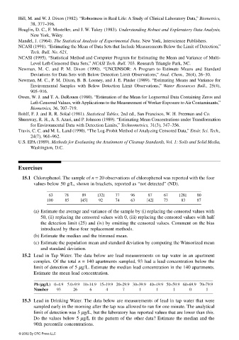
15.1 Chlorophenol. The sample of n = 20 observations of chlorophenol was reported with the four
values below 50 g/L, shown in brackets, reported as “not detected” (ND).
63 78 89 [32] 77 96 87 67 [28] 80
100 85 [45] 92 74 63 [42] 73 83 87
(a) Estimate the average and variance of the sample by (i) replacing the censored values with
50, (ii) replacing the censored values with 0, (iii) replacing the censored values with half
the detection limit (25) and (iv) by omitting the censored values. Comment on the bias
introduced by these four replacement methods.
(b) Estimate the median and the trimmed mean.
(c) Estimate the population mean and standard deviation by computing the Winsorized mean
and standard deviation.
15.2 Lead in Tap Water. The data below are lead measurements on tap water in an apartment
complex. Of the total n = 140 apartments sampled, 93 had a lead concentration below the
limit of detection of 5 µg/L. Estimate the median lead concentration in the 140 apartments.
Estimate the mean lead concentration.

Pb (µµ µµg// //L) 0–4.9 5.0–9.9 10–14.9 15–19.9 20–29.9 30–39.9 40–49.9 50–59.9 60–69.9 70–79.9
Number 93 26 6 4 7 1 1 1 0 1
15.3 Lead in Drinking Water. The data below are measurements of lead in tap water that were
sampled early in the morning after the tap was allowed to run for one minute. The analytical
limit of detection was 5 µg/L, but the laboratory has reported values that are lower than this.
Do the values below 5 µg/L fit the pattern of the other data? Estimate the median and the
90th percentile concentrations.
© 2002 By CRC Press LLC