Page 139 - Statistics for Environmental Engineers

L1592_Frame_C15 Page 136 Tuesday, December 18, 2001 1:50 PM

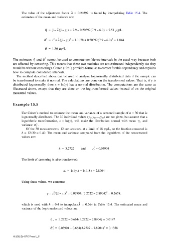
The value of the adjustment factor λ = 0.20392 is found by interpolating Table 15.4. The
ˆ
estimates of the mean and variance are:

(
η ˆ = y λ y –(– ˆ y c ) = 7.9 0.20392 7.9 6.0) = 7.51 µg/L
–
–
(
σ ˆ = s + λ y – y c ) = 1.1078 + 0.20392 7.9 6.0) = 1.844
(
2
2
2
ˆ
2
–
σ ˆ = 1.36 µg L
η ˆ
The estimates and σ ˆ 2 cannot be used to compute confidence intervals in the usual way because both
are affected by censoring. This means that these two statistics are not estimated independently (as they
would be without censoring). Cohen (1961) provides formulas to correct for this dependency and explains
how to compute confidence intervals.
The method described above can be used to analyze lognormally distributed data if the sample can
be transformed to make it normal. The calculations are done on the transformed values. That is, if y is
distributed lognormally, then x = ln y() has a normal distribution. The computations are the same as
illustrated above, except that they are done on the log-transformed values instead of on the original
measured values.
Example 15.5

Use Cohen’s method to estimate the mean and variance of a censored sample of n = 30 that is
lognormally distributed. The 30 individual values (y 1 , y 2 ,…,y 30 ) are not given, but assume that a
logarithmic transformation, x = ln y() , will make the distribution normal with mean η x and
2
variance σ x .
Of the 30 measurements, 12 are censored at a limit of 18 µg/L, so the fraction censored is
h = 12/30 = 0.40. The mean and variance computed from the logarithms of the noncensored
values are:

x = 3.2722 and s x = 0.03904
2

The limit of censoring is also transformed:

()
(
x c = ln y c = ln 18) = 2.8904
Using these values, we compute:

(
(
γ = s x / x – x c ) = 0.03904/ 3.2722 2.8904) = 0.2678.
2
2
2
–
λ
ˆ
which is used with h = 0.4 to interpolate = 0.664 in Table 15.4. The estimated mean and
variance of the log-transformed values are:
(
η ˆ x = 3.2722 0.664 3.2722 2.8904) = 3.0187
–
–
(
2
2 0.03904 + 0.664 3.2722 2.8904) =
σ ˆ x = – 0.1358
© 2002 By CRC Press LLC