Page 143 - Statistics for Environmental Engineers

L1592_Frame_C15 Page 140 Tuesday, December 18, 2001 1:50 PM

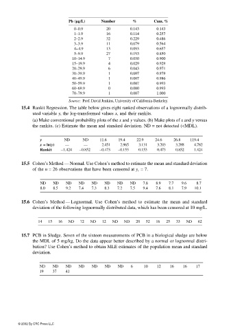
Pb (µg// //L) Number % Cum. %
0–0.9 20 0.143 0.143
1–1.9 16 0.114 0.257
2–2.9 32 0.229 0.486
3–3.9 11 0.079 0.564
4–4.9 13 0.093 0.657
5–9.9 27 0.193 0.850
10–14.9 7 0.050 0.900
15–19.9 4 0.029 0.929
20–29.9 6 0.043 0.971
30–39.9 1 0.007 0.979
40–49.9 1 0.007 0.986
50–59.9 1 0.007 0.993
60–69.9 0 0.000 0.993
70–79.9 1 0.007 1.000
Source: Prof. David Jenkins, University of California-Berkeley.
15.4 Rankit Regression. The table below gives eight ranked observations of a lognormally distrib-
uted variable y, the log-transformed values x, and their rankits.
(a) Make conventional probability plots of the x and y values. (b) Make plots of x and y versus
the rankits. (c) Estimate the mean and standard deviation. ND = not detected (<MDL).

y ND ND 11.6 19.4 22.9 24.6 26.8 119.4
x == == ln(y) — — 2.451 2.965 3.131 3.203 3.288 4.782
Rankit −1.424 −0.852 −0.473 −0.153 0.153 0.473 0.852 1.424

15.5 Cohen’s Method — Normal. Use Cohen’s method to estimate the mean and standard deviation
of the n = 26 observations that have been censored at y c = 7.

ND ND ND ND ND ND ND ND 7.8 8.9 7.7 9.6 8.7
8.0 8.5 9.2 7.4 7.3 8.3 7.2 7.5 9.4 7.6 8.1 7.9 10.1

15.6 Cohen’s Method — Lognormal. Use Cohen’s method to estimate the mean and standard
deviation of the following lognormally distributed data, which has been censored at 10 mg/L.

14 15 16 ND 72 ND 12 ND ND 20 52 16 25 33 ND 62

15.7 PCB in Sludge. Seven of the sixteen measurements of PCB in a biological sludge are below
the MDL of 5 mg/kg. Do the data appear better described by a normal or lognormal distri-
bution? Use Cohen’s method to obtain MLE estimates of the population mean and standard
deviation.

ND ND ND ND ND ND ND 6 10 12 16 16 17
19 37 41

© 2002 By CRC Press LLC