Page 140 - Statistics for Environmental Engineers

L1592_Frame_C15 Page 137 Tuesday, December 18, 2001 1:50 PM

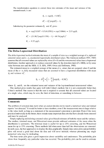
The transformation equations to convert these into estimates of the mean and variance of the
untransformed y’s are:

η ˆ y = exp ( η ˆ x + 0.5σ ˆ x)
2
[
σ ˆ y = η ˆ y exp σ ˆ x) 1]
(
2
2
2
–
2
Substituting the parameter estimatesη ˆ x and σ ˆ x gives:
[
(
η ˆ y = exp 3.0187 + 0.5 0.1358)] = exp ( 3.0866) = 21.9 µg/L
σ ˆ y = ( 21.90) exp 0.1358) 1] = 69.76 µg/L) 2
(
(
[
2
2
–
σ ˆ y = 8.35 µg/L
The Delta-Lognormal Distribution
The delta-lognormal method estimates the mean of a sample of size n as a weighted average of n c replaced
censored values and n – n c uncensored lognormally distributed values. The Aitchison method (1955, 1969)
assumes that all censored values are replaced by zeros (D = 0) and the noncensored values have a lognormal
distribution. Another approach is to replace censored values by the detection limit (D = MDL) or by some
value between zero and the MDL (U.S. EPA, 1989; Owen and DeRouen, 1980).
The estimated mean is a weighted average of the mean of n c values that are assigned value D and the
mean of the n – n c fully measured values that are assumed to have a lognormal distribution with mean
2
η x and variance σ x .
---- exp η ˆ x –(
η ˆ y = D---- +  1 – n c 0.5σ ˆ x )
2
n c
n  n 
are the estimated mean and variance of the log-transformed noncensored values.
where η ˆ x andσ ˆ x
This method gives results that agree well with Cohen’s method, but it is not consistently better than
Cohen’s method. One reason is that the user is required to assume that all censored values are located
at a single value, which may be zero, the limit of detection, or something in between.

Comments
The problem of censored data starts when an analyst decides not to report a numerical value and instead
reports “not detected.” It would be better to have numbers, even if the measurement error is large relative
to the value itself, as long as a statement of the measurement’s precision is provided. Even if this were
practiced universally in the future, there remain many important data sets that have already been censored
and must be analyzed.
Simply replacing and deleting censored values gives biased estimates of both the mean and the variance.
The median, trimmed mean, and Winsorized mean provide unbiased estimates of the mean when the
distribution is symmetric. The trimmed mean is useful for up to 25% censoring, and the Winsorized
mean for up to 15% censoring. These methods fail when more than half the observations are censored.
In such cases, the best approach is to display the data graphically. Simple time series plots and probability
plots will reveal a great deal about the data and will never mislead, whereas presenting any single
numerical value may be misleading.
The time series plot gives a good impression about variability and randomness. The probability plot
shows how frequently any particular value has occurred. The probability plot can be used to estimate

© 2002 By CRC Press LLC