Page 136 - Statistics for Environmental Engineers

L1592_Frame_C15 Page 133 Tuesday, December 18, 2001 1:50 PM

5
4
3 2
Mercury Concentration (µg/L) 0.5 1 MDL = 0.2 µg/L

0.4
0.3
0.2

0.1
0.05
40 50 60 70 80 90 95 98 99
Cumulative Probability

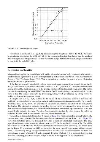
FIGURE 15.2 Cumulative probability plot.

The median is estimated as 0.1 µg/L by extrapolating the straight line below the MDL. We cannot
be certain that data below the MDL will fall on the extrapolated straight line, but at least the available
data do not preclude this possibility. The line was drawn by eye. In the next section, a regression method
is used to fit the probability plot.

Regression on Rankits
It is possible to replace the probabilities with rankits (also called normal order scores or order statistics)
and then to use regression to fit a line to the probability plot (Gilliom and Helsel, 1986; Hashimoto and
Trussell, 1983; Travis and Land, 1990). This is equivalent to rescaling the graph in terms of standard
deviations instead of probabilities.
If the data are normally distributed, or have been transformed to make them normal, the probabili-
ties(p) are converted to rankits (normal order scores),R i = F 1 (p i ) where F −1 is the inverse cumulative
normal probability distribution and p i is the plotting position of the ith ranked observation. The rankits
can be calculated (using the NORMSINV function in EXCEL) or looked up in standard statistical tables
(for n ≤ 50). The analysis could also be done using probits, which are obtained by adding five to the
rankits to eliminate the negative values.
A straight line y i = b 0 + b 1 R i is fitted to the rankits of the noncensored portion of the data. The
rankits(R) are treated as the independent variable and the data are the dependent variable. For normally
distributed data, the b 0 and b 1 are estimates of the mean and standard deviation of the noncensored
distribution. The intercept b 0 estimates the median because rankits are symmetrical about zero and the
50th percentile corresponds to R i = 0. For the normal distribution, the median equals the mean, so the 50th
percentile also estimates the mean. The slope b 1 estimates the standard deviation because the rankits are
scaled so that one rankit is one standard deviation on the original scale.
The method is demonstrated using the 45 values in Table 15.3 (these are random normal values). The
concentrations have been ranked and the rankits are from the tables of Rohlf and Sokal (1981). Figure 15.3
shows the probability plots. The top panel shows the 45 normally distributed observations. The linear
regression of concentration on rankits estimates a mean of 33.3 and a standard deviation of 5.4. The middle
panel shows the result when the 10 smallest observations are censored (22% censoring). The bottom panel
has the lowest 20 values censored (44% censoring) so the mean can still be estimated without extrapo-
lation. The censoring hardly changed the estimates of the mean and standard deviation. All three data
sets estimate a mean of about 33.5 and a standard deviation of about 5. It is apparent, however, that
increased censoring gives more relative weight to values in the upper tail of the distribution.
© 2002 By CRC Press LLC