Page 137 - Statistics for Environmental Engineers

L1592_Frame_C15 Page 134 Tuesday, December 18, 2001 1:50 PM

TABLE 15.3
Censored Data Analysis Using Rankits (Normal Order Statistics)
Conc. Rankit Conc. Rankit Conc. Rankit
23.8 −2.21 31.0 −0.40 36.4 0.46
24.4 −1.81 31.6 −0.34 37.0 0.52
25.0 −1.58 31.6 −0.28 37.0 0.59
25.0 −1.41 31.6 −0.22 37.0 0.65
25.6 −1.27 32.2 −0.17 37.0 0.72
25.6 −1.16 32.8 −0.11 37.0 0.80
28.0 −1.05 33.4 −0.06 37.6 0.88
28.0 −0.96 34.1 0.0 37.6 0.96
28.0 −0.88 34.6 0.06 38.2 1.05
28.6 −0.80 35.2 0.11 38.2 1.16
28.6 −0.72 35.2 0.17 39.4 1.27
29.2 −0.65 35.2 0.22 39.4 1.41
29.8 −0.59 35.8 0.28 40.6 1.58
29.8 −0.52 35.8 0.34 43.6 1.81
31.0 −0.46 35.8 0.40 47.8 2.21

50
all 45 observations 10 values censored 20 values censored
Concentration 40
y = 33.8 + 5.0x
y = 33.6 + 3.6x
y = 33.3 + 5.4x
30
20
-2 -1 0 1 2 -2 -1 0 1 2 -2 -1 0 1 2
Rankit Rankit Rankit

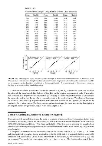
FIGURE 15.3 The left panel shows the rankit plot for a sample of 45 normally distributed values. In the middle panel,
10 values have been censored; the right panel has 20 censored values. Regression with rankits as the independent variables
and concentration as the dependent variables gives the intercept (rankit = 0) as an estimated of the median = mean, and
the slope as an estimate of the standard deviation.

If the data have been transformed to obtain normality, b 0 and b 1 estimate the mean and standard
deviation of the transformed data, but not of the data on the original measurement scale. If normality
was achieved by a logarithmic transformation z =[ ln y()] , the 50th percentile (median of z) estimates
the mean of z and is also the log of the geometric mean in the original metric. The slope will estimate
the standard deviation of z. Exponentiation transforms the median on the log-scale transform to the
median in the original metric. The back transformations to estimate the mean and standard deviation in
the original metric are given in Chapter 7 and in Example 15.5.

Cohen’s Maximum Likelihood Estimator Method
There are several methods to estimate the mean of a sample of censored data. Comparative studies show
that none is always superior so we have chosen to present Cohen’s maximum likelihood method (Cohen,
1959, 1961; Gilliom and Helsel, 1986; Haas and Scheff, 1990). It is easy to compute for samples from
a normally distributed parent population or from a distribution that can be made normal by a log-arithmic
transformation.
A sample of n observations has measured values of the variable only at y ≥ y c , where y c is a known
and fixed point of censoring. In our application, y c is the MDL and it is assumed that the same MDL
applies to each observation. Of the n total observations in the sample, n c observations have y ≤ y c and
are censored. The number of observations with y > y c is k = n n c . The fraction of censored data is
–
© 2002 By CRC Press LLC