Page 151 - Statistics for Environmental Engineers

L1592_frame_C17 Page 148 Tuesday, December 18, 2001 1:51 PM

about the direction of the difference. The standard procedure for making such comparisons is to construct
a null hypothesis that is tested statistically using a t-test. The classical null hypothesis is: “The difference
between the two methods is zero.” We do not expect two methods to give exactly the same results, so it
may seem strange to investigate a hypothesis that is certainly wrong. The philosophy is the same as in
law where the accused is presumed innocent until proven guilty. We cannot prove a person innocent,
which is why the verdict is worded “not guilty” when the evidence is insufficient to convict. In a statistical
comparison, we cannot prove that two methods are the same, but we can collect evidence that shows
them to be different. The null hypothesis is therefore a philosophical device for letting us avoid saying
that two things are equal. Instead we conclude, at some stated level of confidence, that “there is a diffe-
rence” or that “the evidence does not permit me to confidently state that the two methods are different.”
An alternate, but equivalent, approach to constructing a null hypothesis is to compute the difference and
the interval in which the difference is expected to fall if the experiment were repeated many, many times.
This interval is called the confidence interval. For example, we may determine that “A – B = 0.20 and that
the true difference falls in the interval 0.12 to 0.28, this statement being made at a 95% level of confidence.”
This tells us all that is important. We are highly confident that A gives a result that is, on average, higher
than B. And it tells all this without the sometimes confusing notions of null hypothesis and significance tests.

Case Study: Interlaboratory Study of Dissolved Oxygen

An important procedure in certifying the quality of work done in laboratories is the analysis of standard
specimens that contain known amounts of a substance. These specimens are usually introduced into the
laboratory routine in a way that keeps the analysts blind to the identity of the sample. Often the analyst is
blind to the fact that quality assurance samples are included in the assigned work. In this example, the
analysts were asked to measure the dissolved oxygen (DO) concentration of the same specimen using two
different methods.
Fourteen laboratories were sent a test solution that was prepared to have a low dissolved oxygen
concentration (1.2 mg/L). Each laboratory made the measurements using the Winkler method (a titration)
and the electrode method. The question is whether the two methods predict different DO concentrations.
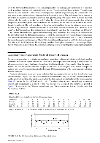
Table 17.1 shows the data (Wilcock et al., 1981). The observations for each method may be assumed
random and independent as a result of the way the test was designed. The differences plotted in
Figure 17.1 suggest that the Winkler method may give DO measurements that are slightly lower than
the electrode method.

TABLE 17.1
Dissolved Oxygen Data from the Interlaboratory Study
Laboratory 1 2 3 4 5 6 7 8 9 10 11 12 13 14
Winkler 1.2 1.4 1.4 1.3 1.2 1.3 1.4 2.0 1.9 1.1 1.8 1.0 1.1 1.4
Electrode 1.6 1.4 1.9 2.3 1.7 1.3 2.2 1.4 1.3 1.7 1.9 1.8 1.8 1.8
Diff. (W – E) −0.4 0.0 −0.5 −1.0 −0.5 0.0 −0.8 0.6 0.6 −0.6 −0.1 −0.8 −0.7 −0.4
Source: Wilcock, R. J., C. D. Stevenson, and C. A. Roberts (1981). Water Res., 15, 321–325.

2
Difference (W – E) 0

-2
1 5 10 14
Laboratory

FIGURE 17.1 The DO data and the differences of the paired values.
© 2002 By CRC Press LLC