Page 155 - Statistics for Environmental Engineers

L1592_frame_C17 Page 152 Tuesday, December 18, 2001 1:51 PM

Density Difference (Inlet - Outlet) -10000
5000
0
-5000

-15000
20000
40000
60000
0
Inlet Copepod Density 80000
Density Difference In (In) - (Out) -0.1
0.3
0.2
0.1
0.0
-0.2
-0.3
8
10
9
11
In (Inlet Copepod Density) 12
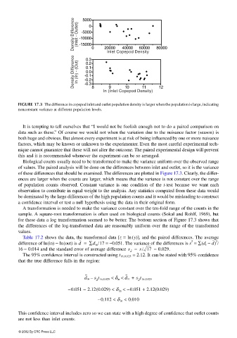
FIGURE 17.3 The difference in copepod inlet and outlet population density is larger when the population is large, indicating
nonconstant variance at different population levels.
It is tempting to tell ourselves that “I would not be foolish enough not to do a paired comparison on
data such as these.” Of course we would not when the variation due to the nuisance factor (season) is
both huge and obvious. But almost every experiment is at risk of being influenced by one or more nuisance
factors, which may be known or unknown to the experimenter. Even the most careful experimental tech-
nique cannot guarantee that these will not alter the outcome. The paired experimental design will prevent
this and it is recommended whenever the experiment can be so arranged.
Biological counts usually need to be transformed to make the variance uniform over the observed range
of values. The paired analysis will be done on the differences between inlet and outlet, so it is the variance
of these differences that should be examined. The differences are plotted in Figure 17.3. Clearly, the differ-
ences are larger when the counts are larger, which means that the variance is not constant over the range
of population counts observed. Constant variance is one condition of the t-test because we want each
observation to contribute in equal weight to the analysis. Any statistics computed from these data would
be dominated by the large differences of the high population counts and it would be misleading to construct
a confidence interval or test a null hypothesis using the data in their original form.
A transformation is needed to make the variance constant over the ten-fold range of the counts in the
sample. A square-root transformation is often used on biological counts (Sokal and Rohlf, 1969), but
for these data a log transformation seemed to be better. The bottom section of Figure 17.3 shows that
the differences of the log-transformed data are reasonably uniform over the range of the transformed
values.
Table 17.2 shows the data, the transformed data [z = ln(y)], and the paired differences. The average
2
difference of ln(in) − ln(out) is d = ∑d in /17 = −0.051. The variance of the differences is s = ∑(d i − ) /d 2
16 = 0.014 and the standard error of average difference s = s/ 17 = 0.029.
d
The 95% confidence interval is constructed using t 16,0.025 = 2.12. It can be stated with 95% confidence
that the true difference falls in the region:

d ln – s t 16,0.025 < δ ln < d ln + s t 16,0.025
d d
−0.051 − 2.12(0.029) < δ ln < −0.051 + 2.12(0.029)
−0.112 < δ ln < 0.010

This confidence interval includes zero so we can state with a high degree of confidence that outlet counts
are not less than inlet counts.

© 2002 By CRC Press LLC