Page 160 - Statistics for Environmental Engineers

L1592_frame_C18.fm Page 158 Tuesday, December 18, 2001 1:52 PM

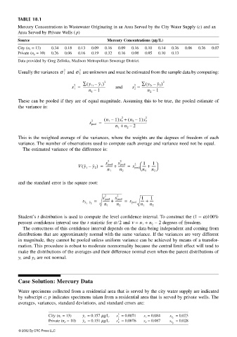
TABLE 18.1
Mercury Concentrations in Wastewater Originating in an Area Served by the City Water Supply (c) and an
Area Served by Private Wells ( p)
Source Mercury Concentrations (µµ µµg/L)
City (n c = 13) 0.34 0.18 0.13 0.09 0.16 0.09 0.16 0.10 0.14 0.26 0.06 0.26 0.07
Private (n p = 10) 0.26 0.06 0.16 0.19 0.32 0.16 0.08 0.05 0.10 0.13
Data provided by Greg Zelinka, Madison Metropolitan Sewerage District.
2 2
Usually the variances σ 1 and σ 2 are unknown and must be estimated from the sample data by computing:
(
(
s 1 = ∑ y 1i – y 1 ) 2 and s 2 = ∑ y 2i – y 2 ) 2
2
2
----------------------------
----------------------------
n 1 – 1 n 2 – 1
These can be pooled if they are of equal magnitude. Assuming this to be true, the pooled estimate of
the variance is:
( n 1 – 1)s 1 + ( n 2 – 2
2
s pool = -----------------------------------------------------
2
1)s 2
n 1 + n 2 – 2
This is the weighted average of the variances, where the weights are the degrees of freedom of each
variance. The number of observations used to compute each average and variance need not be equal.
The estimated variance of the difference is:
2 2
2 
1
1
Vy 1 –( y 2 ) = -------- + -------- = s pool ----- + -----  
s pool
s pool

n 1 n 2 n 1 n 2
and the standard error is the square root:
2 2
1
1
= -------- + -------- = s pool ----- + -----
s pool
s pool
s y 1 −y 2
n 1 n 2 n 1 n 2
Student’s t distribution is used to compute the level confidence interval. To construct the (1 − α)100%
percent confidence interval use the t statistic for α /2 and ν = n 1 + n 2 − 2 degrees of freedom.
The correctness of this confidence interval depends on the data being independent and coming from
distributions that are approximately normal with the same variance. If the variances are very different
in magnitude, they cannot be pooled unless uniform variance can be achieved by means of a transfor-
mation. This procedure is robust to moderate nonnormality because the central limit effect will tend to
make the distributions of the averages and their difference normal even when the parent distributions of
y 1 and y 2 are not normal.

Case Solution: Mercury Data
Water specimens collected from a residential area that is served by the city water supply are indicated
by subscript c; p indicates specimens taken from a residential area that is served by private wells. The
averages, variances, standard deviations, and standard errors are:

2
City (n c = 13) y c = 0.157 µg/L s c = 0.0071 s c = 0.084 s y c = 0.023
2
Private (n p = 10) y p = 0.151 µg/L s p = 0.0076 s p = 0.087 s y p = 0.028
© 2002 By CRC Press LLC