Page 165 - Statistics for Environmental Engineers

L1592_frame_C19.fm Page 163 Tuesday, December 18, 2001 1:53 PM

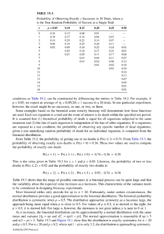
TABLE 19.3
Probability of Observing Exactly x Successes in 20 Trials, where p
is the True Random Probability of Success in a Single Trial
x p == == 0.05 0.10 0.15 0.20 0.25 0.50
0 0.36 0.12 0.04 0.01 — —
1 0.38 0.27 0.14 0.06 0.02 —
2 0.18 0.29 0.22 0.14 0.07 —
3 0.06 0.19 0.25 0.20 0.14 —
4 0.02 0.09 0.18 0.22 0.18 0.01
5 0.03 0.10 0.17 0.21 0.01
6 0.01 0.05 0.11 0.17 0.04
7 0.01 0.06 0.11 0.07
8 0.01 0.02 0.06 0.12
9 0.01 0.02 0.16
10 0.01 0.18
11 0.16
12 0.12
13 0.07
14 0.04
15 0.01
16 0.01

conditions as Table 19.2, can be constructed by differencing the entries in Table 19.2. For example, if
p = 0.05, we expect an average of η x = 0.05(20) = 1 success in a 20 trials. In one particular experiment,
however, the result might be no successes, or one, or two, or three.
Some examples based on the binomial acute toxicity bioassay will demonstrate how these functions
are used. Each test organism is a trial and the event of interest is its death within the specified test period.
It is assumed that (1) theoretical probability of death is equal for all organisms subjected to the same
treatment and (2) the fate of each organism is independent of the fate of other organisms. If n organisms
are exposed to a test condition, the probability of observing any specific number of dead organisms,
given a true underlying random probability of death for an individual organism, is computed from the
binomial distribution.
From Table 19.2, the probability of getting one or no deaths is Pr(x ≤ 1) = 0.74. From Table 19.3, the
probability of observing exactly zero deaths is Pr(x = 0) = 0.36. These two values are used to compute
the probability of exactly one death:
(
(
(
Pr x = 1) = Pr x ≤ 1) Pr x ≤ 0) = 0.74 0.36 = 0.38
–
–
This is the value given in Table 19.3 for x = 1 and p = 0.05. Likewise, the probability of two or less
deaths is Pr(x ≤ 2) = 0.92 and the probability of exactly two deaths is:
(
(
Pr x = 2) = Pr x ≤ 2) Pr x ≤ 1) = 0.92 0.74 = 0.18
(
–
–
Table 19.3 shows that the range of possible outcomes in a binomial process can be quite large and that
the variability about the expected value increases as p increases. This characteristic of the variance needs
to be considered in designing bioassay experiments.
Most binomial tables only provide for up to n = 20. Fortunately, under certain circumstances, the
normal distribution provides a good approximation to the binomial distribution. The binomial probability
distribution is symmetric when p = 0.5. The distribution approaches symmetry as n becomes large, the
approach being more rapid when p is close to 0.5. For values of p ≤ 0.5, it is skewed to the right; for
p > 0.5, it is skewed left. For large n, however, the skewness is not great unless p is near to 0 or 1.
As n increases, the binomial distribution can be approximated by a normal distribution with the same
2
mean and variance [η x = np and σ x = np(1 − p)]. The normal approximation is reasonable if np > 5
and n(1 − p) > 5. Table 19.3 and Figure 19.1 show that the distribution is exactly symmetric for n = 20
and p = 0.5. For n = 20 and p = 0.2, where np(1 − p) is only 3.2, the distribution is approaching symmetry.
© 2002 By CRC Press LLC