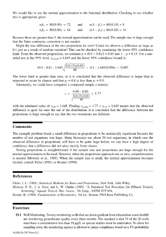
Page 168 - Statistics for Environmental Engineers

L1592_frame_C19.fm Page 166 Tuesday, December 18, 2001 1:53 PM

We would like to use the normal approximation to the binomial distribution. Checking to see whether
this is appropriate gives:

np ˆ 1 = 80 0.90) = 72 and n 1 – p ˆ 1 ) = 80 0.10) = 8
(
(
(
(
(
np ˆ 2 = 80 0.80) = 64 and n 1 – p ˆ 2 ) = 80 0.20) = 16
(
Because these are greater than 5, the normal approximation can be used. The sample size is large enough
that the Yates continuity correction is not needed.
Might the true difference of the two proportions be zero? Could we observe a difference as large as
0.1 just as a result of random variation? This can be checked by examining the lower 95% confidence
limit. From the observed proportions, we estimate p = (0.9 + 0.8)/2 = 0.85 and 1 − p = 0.15. For a one-
sided test at the 95% level, z α=0.05 = 1.645 and the lower 95% confidence bound is:
2 0.15) 0.85)
(
(
( 0.9 0.8) 1.645 ----------------------------------– = 0.1 1.645 0.056) = 0.007
(
–
–
80
The lower limit is greater than zero, so it is concluded that the observed difference is larger than is
expected to occur by chance and that p 2 = 0.8 is less than p 1 = 0.9.
Alternately, we could have compared a computed sample z-statistic:
–
0.90 0.80
z = -------------------------------- = 1.77
2 0.15) 0.85)
(
(
----------------------------------
80
with the tabulated value of z 0.05 = 1.645. Finding z sample = 1.77 > z 0.05 = 1.645 means that the observed
difference is quite far onto the tail of the distribution. It is concluded that the difference between the
proportions is large enough to say that the two treatments are different.
Comments

The example problem found a small difference in proportions to be statistically significant because the
number of test organisms was large. Many bioassays use about 20 test organisms, in which case the
observed difference in proportions will have to be quite large before we can have a high degree of
confidence that a difference did not arise merely from chance.
Testing proportions is straightforward if the sample size and proportions are large enough for the
normal approximation to be used. However, when the proportions approach one or zero, a transformation
is needed (Mowery et al., 1985). When the sample size is small, the normal approximation becomes
invalid; consult Fleiss (1981) or Rosner (1990).

References

Fleiss, J. L. (1981). Statistical Methods for Rates and Proportions, New York, John Wiley.
Mowery, P. D., J. A. Fava, and L. W. Clatlin (1985). “A Statistical Test Procedure for Effluent Toxicity
Screening,” Aquatic Toxicol. Haz. Assess., 7th Symp., ASTM STP 854.
Rosner, B. (1990). Fundamentals of Biostatistics, 3rd ed., Boston, PWS-Kent Publishing Co.

Exercises
19.1 Well Monitoring. Twenty monitoring wells that are down-gradient from a hazardous waste landfill
are monitoring groundwater quality every three months. The standard is that 19 of the 20 wells
must have a concentration less than 10 µg/L or special studies must be undertaken. To allow for
sampling error, the monitoring agency is allowed to judge compliance based on a 5% probability
© 2002 By CRC Press LLC