Page 167 - Statistics for Environmental Engineers

L1592_frame_C19.fm Page 165 Tuesday, December 18, 2001 1:53 PM

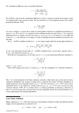
The standardized difference also is normally distributed:
( p ˆ 1 – p ˆ 2 ) 0
–
z = ----------------------------------------------

1 
1
(
p 1 – p) ----- + -----
n 

2
n 1
The difficulty with using the standardized difference is that p is unknown and the denominator cannot
be computed until some estimate is found. The best estimate of p is the weighted average of the sample
proportions (Rosner, 1990):
n 1 p ˆ 1 +
p = ---------------------------
n 2 p ˆ 2
n 1 + n 2
Use this to compute z as given above under the null hypothesis that the two population proportions are
equal (p 1 = p 2 ). This value of z is compared with the tabulated standard normal variate, z α , for a specified
significance level α. Usually only the case where p 1 > p 2 (or p 2 > p 1 ) is of interest, so a one-sided test
is used. If z > z α , the difference is too large to accept the hypothesis that the population proportions are
the same.
The (1 − α)100% confidence limits for p 1 − p 2 for a large sample under the normal approximation is:

p ˆ 1 )
p ˆ 2 1 –(
(
p ˆ 2 )
p ˆ 1 1 –
p ˆ 1 – p ˆ 2 ± z α/2 ------------------------- + -------------------------
n 1 n 2
To set a one-sided upper bound with a (1 − α)100% confidence level, use the above equation with z α .
To set a one-sided lower bound, use −z α .
When the two test populations are the same size (n = n 1 = n 2 ), the standardized difference simplifies to:
( p ˆ 1 – p ˆ 2 ) 0
–
z = ------------------------------
(
2 p 1 – p)
------------------------
n
where p = (p ˆ 1 + p ˆ 2 )/2.
Fleiss (1981) suggests that when n is small (e.g., n < 20), the computation of z should be modified to:
( p ˆ 1 – p ˆ 2 ) – 1 ---
z = ------------------------------ n
(
2 p 1 – p)
------------------------
n
The (−1/n) in the numerator is the Yates continuity correction, which takes into account the fact that a
continuous distribution (the normal) is being used to represent the discrete binomial distribution of
sample proportions. For reasonably small n (e.g., n = 20), the correction is −1/n = −0.05, which can be
substantial relative to the differences usually observed (e.g., p 1 − p 2 = 0.15). Not everyone uses this
correction (Rosner, 1990). If it is omitted, there is a reduced probability of detecting a difference in
rates. As n becomes large, this correction factor becomes negligible because the normal distribution very
closely approximates the binomial distribution.

Case Study Solution

Eighty organisms (n 1 = n 1 = 80) were exposed to each treatment condition (control and effluent) and the
sample survival proportions are observed to be:
p ˆ 1 = 72/80 = 0.90 and p ˆ 2 = 64/80 = 0.80

© 2002 By CRC Press LLC