Page 154 - Statistics for Environmental Engineers

L1592_frame_C17 Page 151 Tuesday, December 18, 2001 1:51 PM

A t-test on the difference of the averages would conclude that A and B are not different. The reason
is that the variance of the averages over M, W, and F is inflated by the day-to-day variation. This day-
to-day variation overwhelms the analysis; pairing removes the problem.
The experimenter who does not think of pairing (blocking) the experiment works at a tremendous
handicap and will make many wrong decisions. Imagine that the collecting for A was done on M, W,
F, of one week and collection for B was done in another week. Now the paired analysis cannot be done
and the difference will not be detected. This is why we speak of a paired design as well as of a paired
t-test analysis. The crucial step is making the correct design. Pairing is always recommended.

Case Study to Emphasize the Benefits of a Paired Design
A once-through cooling system at a power plant is suspected of reducing the population of certain aquatic
organisms. The copepod population density (organisms per cubic meter) were measured at the inlet and
outlet of the cooling system on 17 different days (Simpson and Dudaitis, 1981). On each sampling day,
water specimens were collected within a short time interval, first at the inlet and then at the outlet. The
sampling plan represents a thoughtful effort to block out the effect of day-to-day and month-to-month
variations in population counts. It pairs the inlet and outlet measurements. Of course, it is impossible
to sample the same parcel of water at the inlet and outlet (i.e., the pairing is not exact), but any variation
caused by this will be reflected as a component of the random measurement error.
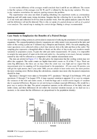
The data are plotted in Figure 17.2. The plot gives the impression that the cooling system may not
affect the copepods. The outlet counts are higher than inlets counts on 10 of the 17 days. There are
some big differences, but these are on days when the count was very high and we expect that the
measurement error in counting will be proportional to the population. (If you count 10 pennies you
will get the right answer, but if you count 1000, you are certain to have some error; the more pennies
the more counting error.) Before doing the calculations, consider once more why the paired comparison
should be done.
Specimens 1 through 6 were taken in November 1977, specimens 7 through 12 in February 1978, and
specimens 13 through 17 in August 1978. A large seasonal variation is apparent. If we were to compute
the variances of the inlet and outlet counts, it would be huge and it would consist largely of variation
due to seasonal differences. Because we are not trying to evaluate seasonal differences, this would be a
poor way to analyze the data. The paired comparison operates on the differences of the daily inlet and
outlet counts, and these differences do not reflect the seasonal variation (except, as we shall see in a
moment, to the extent that the differences are proportional to the population density).

80000
Outlet
Copepod Density 60000
Inlet

40000

20000

0
1 2 3 4 5 6 7 8 9 10 11 12 13 14 15 16 17
Sample

3
FIGURE 17.2 Copepod population density (organisms/m ).
© 2002 By CRC Press LLC