Page 270 - Statistics for Environmental Engineers

L1592_Frame_C30 Page 273 Tuesday, December 18, 2001 2:49 PM

Method
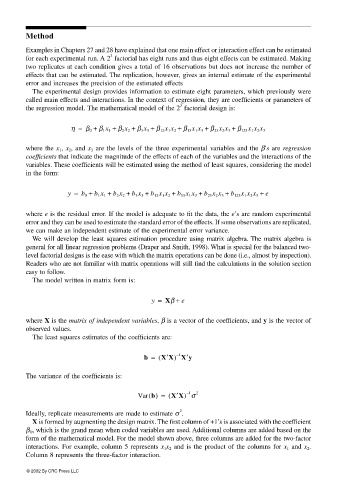
Examples in Chapters 27 and 28 have explained that one main effect or interaction effect can be estimated
3
for each experimental run. A 2 factorial has eight runs and thus eight effects can be estimated. Making
two replicates at each condition gives a total of 16 observations but does not increase the number of
effects that can be estimated. The replication, however, gives an internal estimate of the experimental
error and increases the precision of the estimated effects
The experimental design provides information to estimate eight parameters, which previously were
called main effects and interactions. In the context of regression, they are coefficients or parameters of
3
the regression model. The mathematical model of the 2 factorial design is:
η = β 0 + β 1 x 1 + β 2 x 2 + β 3 x 3 + β 12 x 1 x 2 + β 13 x 1 x 3 + β 23 x 2 x 3 + β 123 x 1 x 2 x 3

where the x 1 , x 2 , and x 3 are the levels of the three experimental variables and the β’s are regression
coefficients that indicate the magnitude of the effects of each of the variables and the interactions of the
variables. These coefficients will be estimated using the method of least squares, considering the model
in the form:

y = b 0 + b 1 x 1 + b 2 x 2 + b 3 x 3 + b 12 x 1 x 2 + b 13 x 1 x 3 + b 23 x 2 x 3 + b 123 x 1 x 2 x 3 + e

where e is the residual error. If the model is adequate to fit the data, the e’s are random experimental
error and they can be used to estimate the standard error of the effects. If some observations are replicated,
we can make an independent estimate of the experimental error variance.
We will develop the least squares estimation procedure using matrix algebra. The matrix algebra is
general for all linear regression problems (Draper and Smith, 1998). What is special for the balanced two-
level factorial designs is the ease with which the matrix operations can be done (i.e., almost by inspection).
Readers who are not familiar with matrix operations will still find the calculations in the solution section
easy to follow.
The model written in matrix form is:

y = Xβ + e

where X is the matrix of independent variables, β is a vector of the coefficients, and y is the vector of
observed values.
The least squares estimates of the coefficients are:

b = ( X′X) X′y
–
1
The variance of the coefficients is:

Var b() = ( X′X) σ 2
–
1
2
Ideally, replicate measurements are made to estimate σ .
X is formed by augmenting the design matrix. The first column of +1’s is associated with the coefficient
β 0 , which is the grand mean when coded variables are used. Additional columns are added based on the
form of the mathematical model. For the model shown above, three columns are added for the two-factor
interactions. For example, column 5 represents x 1 x 2 and is the product of the columns for x 1 and x 2 .
Column 8 represents the three-factor interaction.

© 2002 By CRC Press LLC