Page 272 - Statistics for Environmental Engineers

L1592_Frame_C30 Page 275 Tuesday, December 18, 2001 2:49 PM

These matrices are easy to create and manipulate for a factorial experimental design. X is an orthogonal
matrix, that is, the inner product of any two columns of vectors is zero. Because X is an orthogonal matrix,
X′X is a diagonal matrix, that is, all elements are zero except diagonal elements. If X has n columns
and m rows, X′ has m columns and n rows. The product X′X will be a square matrix with n rows and
−1
n columns. If X′X is a diagonal matrix, its inverse (X′X) is just the reciprocal of the elements of X′X.

Case Study Solution

The variability of the nitrate measurements is larger at the higher concentrations. This is because the
logarithmic scale of the instrument makes it possible to read to 0.1 mg/L at the low concentration but
only to 1 mg/L at the high level. The result is that the measurement errors are proportional to the
measured concentrations. The appropriate transformation to stabilize the variance in this case is to use
the natural logarithm of the measured values. Each value was transformed by taking its natural logarithm
and then the logs of the replicates were averaged.

Parameter Estimation
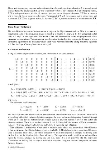
Using the matrix algebra defined above, the coefficients b are calculated as:

1/8 0 0 0 0 0 0 0 1 1 1 1 1 1 1 1 1.0472
0 1/8 0 0 0 0 0 0 – 1 1 – 1 1 – 1 1 – 1 1 3.2770
0 0 1/8 0 0 0 0 0 – 1 – 1 1 1 – 1 – 1 11 1.0805
b = 0 0 0 1/8 0 0 0 0 – 1 – 1 – 1 – 1 1 1 1 1 3.4335
0 0 0 0 1/8 0 0 0 1 – 1 – 1 1 1 – 1 – 1 1 1.0817
0 0 0 0 0 1/8 0 0 1 – 1 1 – 1 – 1 1 – 1 1 3.3140
0 0 0 0 0 0 1/8 0 1 1 – 1 – 1 – 1 – 1 11 1.1627
0 0 0 0 0 0 0 1/8 – 1 1 1 – 1 1 – 1 – 1 1 3.4258
which gives:

b 0 = 1/8 1.0472 + 3.2770 + … + 1.1627 + 3.4258) = 2.2278
(
b 1 = 1/8 – 1.0472 + 3.2770 1.0805 + 3.4335 1.0817 + 3.3140 1.1627 + 3.4258) = 1.1348
(
–
–
–
b 2 = 1/8 −1.0472 3.2770 + 1.0805 + 3.4335 1.0817 3.3140 + 1.1627 + 3.4258) = 0.0478
(
–
–
–
and so on.
The estimated coefficients are:
b 0 = 2.2278 b 1 = 1.1348 b 2 = 0.0478 b 3 = 0.0183
b 12 = 0.0192 b 13 = – 0.0109 b 23 = 0.0004 b 123 = – 0.0115
The subscripts indicate which factor or interaction the coefficient multiplies in the model. Because we
are working with coded variables, b 0 is the average of the observed values. Intrepreting b 0 as the intercept
where all x’s are zero is mathematically correct, but it is physical nonsense. Two of the factors are
discrete variables. There is no method between A and B. Using half the amount of PMA preservative
(i.e., x 2 = 0) would either be effective or ineffective; it cannot be half-effective.
This arithmetic is reminiscent of that used to estimate main effects and interactions. One difference
is that in estimating the effects, division is by 4 instead of by 8. This is because there were four differences
used to estimate each effect. The effects indicate how much the response is changed by moving from
the low level to the high level (i.e., from −1 to +1). The regression model coefficients indicated how
much the response changes by moving one unit (i.e., from −1 to 0 or from 0 to +1). The regression
coefficients are exactly half as large as the effects estimated using the standard analysis of two-level
factorial designs.
© 2002 By CRC Press LLC