Page 358 - Statistics for Environmental Engineers

L1592_Frame_C41 Page 368 Tuesday, December 18, 2001 3:24 PM

This means that when we do not recognize and account for positive autocorrelation, the estimated
2 2
σ a
variance σ e will be larger than the true variance of the random independent errors ( ) by the factor
2 2 2
1/(1 − ρ ). This inflation can be impressive. If ρ is large (i.e., ρ = 0.8), σ e = 2.8σ a .

An Example of Autocorrelated Errors

The laboratory data presented for the case study were created to illustrate the consequences of autocor-
relation on regression. The true model of the experiment is η = 20 + 0.5x. The data structure is shown
in Table 41.1. If there were no autocorrelation, the observed values would be as shown in Figure 41.2.
These are the third column in Table 41.1, which is computed as y i + 20 + 0.5x i + a i , where the a i are
independent values drawn randomly from a normal distribution with mean zero and variance of one (the
a t ’s actually selected have a variance of 1.00 and a mean of −0.28).
In the flawed experiment, hidden factors in the experiment were assumed to introduce autocorrelation.
The data were computed assuming that the experiment generated errors having first-order autocorrelation
with ρ = 0.8. The last three columns in Table 41.1 show how independent random errors are converted
to correlated errors. The function producing the flawed data is:

y i = η + e i = 20 + 0.5x i + 0.8e i−1 + a i

If the data were produced by the above model, but we were unaware of the autocorrelation and fit the
simpler model η = β 0 + β 0 x, the estimates of β 0 and β 1 will reflect this misspecification of the model.
Perhaps more serious is the fact that t-tests and F-tests on the regression results will be wrong, so we
may be misled as to the significance or precision of estimated values. Fitting the data produced from
the autocorrelation model of the process gives y i = 21.0 + 0.12x i . The 95% confidence interval of the
slope is [−0.12 to 0.35] and the t-ratio for the slope is 1.1. Both of these results indicate the slope is not
significantly different from zero. Although the result is reported as statistically insignificant, it is wrong
because the true slope is 0.5.
This is in contrast to what would have been obtained if the experiment had been conducted in a way
that prevented autocorrelation from entering. The data for this case are listed in the “no autocorrelation”
section of Table 41.1 and the results are shown in Table 41.2. The fitted model is y i = 20.06 + 0.43x i ,
the confidence interval of the slope is [0.21 to 0.65] and the t-ratio for the slope is 4.4. The slope is
statistically significant and the true value of the slope (β = 0.5) falls within the confidence interval.
Table 41.2 summarizes the results of these two regression examples ( ρ = 0 and ρ = 0.8). The Durbin-
Watson statistic (explained in the next section) provided by the regression program indicates indepen-
dence in the case where ρ = 0, and shows serial correlation in the other case.

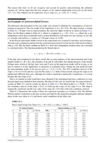
TABLE 41.1
Data Created Using True Values of y i = 20 + 0.5x i + a i with a i = N(0,1)
No Autocorrelation Autocorrelation, ρρ ρρ == == 0.8
x ηη ηη a i y i == == ηη ηη ++ ++ a i 0.8e i−− −−1 ++ + + a i == = = e i y i == == ηη ηη ++ ++ e i
0 20.0 1.0 21.0 0.00 + 1.0 = 1.0 21.0
1 20.5 0.5 21.0 0.80 + 0.5 = 1.3 21.8
2 21.0 –0.7 20.3 1.04 + –0.7 = 0.3 21.3
3 21.5 0.3 21.8 0.27 + 0.3 = 0.6 22.1
4 22.0 0.0 22.0 0.46 + 0.0 = 0.5 22.5
5 22.5 –2.3 20.2 0.37 + –2.3 = –1.9 20.6
6 23.0 –1.9 21.1 –1.55 + –1.9 = –3.4 19.6
7 23.5 0.2 23.7 –2.76 + 0.2 = –2.6 20.9
8 24.0 –0.3 23.7 –2.05 + –0.3 = –2.3 21.7
9 24.5 0.2 24.7 –1.88 + 0.2 = –1.7 22.8
10 25.0 –0.1 24.9 –1.34 + –0.1 = –1.4 23.6

© 2002 By CRC Press LLC