Page 172 - The Mechatronics Handbook

0066-frame-C09 Page 46 Friday, January 18, 2002 11:01 AM

ω
z
I:I x
h ω
T x x
x x 1
h ω h ω
side z y y z
view z h h
z y
G G
Induced T T
torque y ω ω z
back y z
view 1 1
y G
h
ω y h ω
y
z I:I y x z I:I z
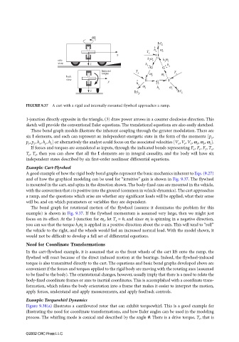
FIGURE 9.37 A cart with a rigid and internally mounted flywheel approaches a ramp.
1-junction directly opposite in the triangle, (3) draw power arrows in a counter clockwise direction. This
sketch will provide the conventional Euler equations. The translational equations are also easily sketched.
These bond graph models illustrate the inherent coupling through the gyrator modulation. There are
six I elements, and each can represent an independent energetic state in the form of the momenta [p x ,
p y , p z , h x , h y , h z ] or alternatively the analyst could focus on the associated velocities [V x , V y , V z , ω x , ω y , ω z ].
If forces and torques are considered as inputs, through the indicated bonds representing F x , F y , F z , T x ,
T y , T z , then you can show that all the I elements are in integral causality, and the body will have six
independent states described by six first-order nonlinear differential equations.
Example: Cart-Flywheel
A good example of how the rigid body bond graphs represent the basic mechanics inherent to Eqs. (9.27)
and of how the graphical modeling can be used for “intuitive” gain is shown in Fig. 9.37. The flywheel
is mounted in the cart, and spins in the direction shown. The body-fixed axes are mounted in the vehicle,
with the convention that z is positive into the ground (common in vehicle dynamics). The cart approaches
a ramp, and the questions which arise are whether any significant loads will be applied, what their sense
will be, and on which parameters or variables they are dependent.
The bond graph for rotational motion of the flywheel (assume it dominates the problem for this
example) is shown in Fig. 9.37. If the flywheel momentum is assumed very large, then we might just
focus on its effect. At the 1-junction for ω x , let T x = 0, and since ω z is spinning in a negative direction,
you can see that the torque h z ω y is applied in a positive direction about the x-axis. This will tend to “roll”
the vehicle to the right, and the wheels would feel an increased normal load. With the model shown, it
would not be difficult to develop a full set of differential equations.
Need for Coordinate Transformations
In the cart-flywheel example, it is assumed that as the front wheels of the cart lift onto the ramp, the
flywheel will react because of the direct induced motion at the bearings. Indeed, the flywheel-induced
torque is also transmitted directly to the cart. The equations and basic bond graphs developed above are
convenient if the forces and torques applied to the rigid body are moving with the rotating axes (assumed
to be fixed to the body). The orientational changes, however, usually imply that there is a need to relate the
body-fixed coordinate frames or axes to inertial coordinates. This is accomplished with a coordinate trans-
formation, which relates the body orientation into a frame that makes it easier to interpret the motion,
apply forces, understand and apply measurements, and apply feedback controls.
Example: Torquewhirl Dynamics
Figure 9.38(a) illustrates a cantilevered rotor that can exhibit torquewhirl. This is a good example for
illustrating the need for coordinate transformations, and how Euler angles can be used in the modeling
process. The whirling mode is conical and described by the angle θ. There is a drive torque, T s , that is

©2002 CRC Press LLC