Page 176 - The Mechatronics Handbook

0066-frame-C09 Page 50 Friday, January 18, 2002 11:01 AM

The terms ∑ l λ l a lk can be interpreted as generalized forces of constraint. These are still workless constraints.
The Lagrange equations for nonholonomic constraints can be used to study holonomic systems, and this
analysis would provide a solution for the constraint forces through evaluation of the Lagrange multipliers.
The use of Lagrange’s equations with Lagrange multipliers is one way to model complex, constrained
multibody systems, as discussed in Haug [14].

Mechanical Subsystem Models Using Lagrange Methods
The previous sections summarize a classical formulation and application of Lagrange’s equations. When
formulating models of mechanical systems, these methods are well proven. Lagrange’s equations are
recognized as an approach useful in handling systems with complex mechanical systems, including systems
with constraints. The energy-basis also makes the method attractive from the standpoint of building multi-
energetic system models, and Lagrange’s equations have been used extensively in electromechanics model-
ing, for example. For conservative systems, it is possible to arrive at solutions sometimes without worrying
about forces, especially since nonconservative effects can be handled “outside” the conservative dynamics.
Developing transformation equations between the coordinates, say x, used to describe the system and the
independent coordinates, q, helps assure a minimal formulation. However, it is possible sometimes to lose
insight into cause and effect, which is more evident in other approaches. Also, the algebraic burden can
become excessive. However, it is the analytical basis of the method that makes it especially attactive. Indeed,
with computer-aided symbolic processing techniques, extensive algebra becomes a non-issue.
In this section, the advantages of the Lagrange approach are merged with those of a bond graph
approach. The concepts and formulations are classical in nature; however, the graphical interpretation
adds to the insight provided. Further, the use of bond graphs assures a consistent formulation with
causality so that some insight is provided into how the conservative dynamics described by the energy
functions depend on inputs, which typically arrive from the nonconservative dynamics. The latter are
very effectively dealt with using bond graph methods, and the combined approach is systematic and
yields first-order differential equations, rather than the second-order ODEs in the classical approach.
Also, it will be shown that in some cases the combined approach makes it relatively easy to model certain
systems that would be very troublesome for a direct approach by either method independently.
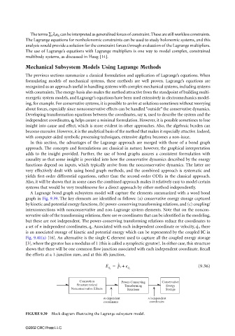
A Lagrange bond graph subsystem model will capture the elements summarized with a word bond
graph in Fig. 9.39. The key elements are identified as follows: (a) conservative energy storage captured
by kinetic and potential energy functions, (b) power-conserving transforming relations, and (c) coupling/
interconnections with nonconservative and non-Lagrange system elements. Note that on the noncon-
servative side of the transforming relations, there are m coordinates that can be identified in the modeling,
but these are not independent. The power-conserving transforming relations reduce the coordinates to
a set of n independent coordinates, q i . Associated with each independent coordinate or velocity, , thereq ˙ i
is an associated storage of kinetic and potential energy which can be represented by the coupled IC in
Fig. 9.40(a) [16]. An alternative is the single C element used to capture all the coupled energy storage
[3], where the gyrator has a modulus of 1 (this is called a symplectic gyrator). In either case, this structure
shows that there will be one common flow junction associated with each independent coordinate. Recall
the efforts at a 1-junction sum, and at this ith junction,

E q = p ˜ i + (9.36)
˙
i e q i
Connection Power-Conserving Conservative
Structure to/and Transforming Energy
Nonconservative Effects Relations Storage

m dependent n independent
coordinates coordinates

FIGURE 9.39 Block diagram illustrating the Lagrange subsystem model.

©2002 CRC Press LLC