Page 178 - The Mechatronics Handbook

0066-frame-C09 Page 52 Friday, January 18, 2002 11:01 AM

1 q
q 1
q x 1 1
TF 1
x 1 q 1 1 TF
x m q n x 2
q 2
1
x 3
(a) (b)
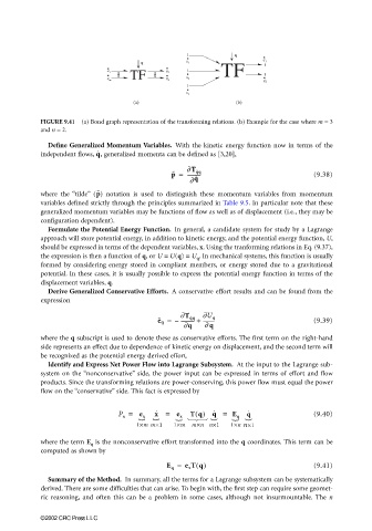
FIGURE 9.41 (a) Bond graph representation of the transforming relations. (b) Example for the case where m = 3
and n = 2.
Define Generalized Momentum Variables. With the kinetic energy function now in terms of the
q ˙ ,
independent flows, generalized momenta can be defined as [3,20],
p ˜ = ∂T ˙ qq (9.38)
-----------
∂ q ˙
p ˜
where the “tilde” ( ) notation is used to distinguish these momentum variables from momentum
variables defined strictly through the principles summarized in Table 9.5. In particular note that these
generalized momentum variables may be functions of flow as well as of displacement (i.e., they may be
configuration dependent).
Formulate the Potential Energy Function. In general, a candidate system for study by a Lagrange
approach will store potential energy, in addition to kinetic energy, and the potential energy function, U,
should be expressed in terms of the dependent variables, x. Using the tranforming relations in Eq. (9.37),
the expression is then a function of q, or U = U(q) = U q . In mechanical systems, this function is usually
formed by considering energy stored in compliant members, or energy stored due to a gravitational
potential. In these cases, it is usually possible to express the potential energy function in terms of the
displacement variables, q.
Derive Generalized Conservative Efforts. A conservative effort results and can be found from the
expression

e ˜ q = – ∂T ˙ qq ∂U q (9.39)
----------- +
---------
∂q ∂ q
where the q subscript is used to denote these as conservative efforts. The first term on the right-hand
side represents an effect due to dependence of kinetic energy on displacement, and the second term will
be recognized as the potential energy derived effort.
Identify and Express Net Power Flow into Lagrange Subsystem. At the input to the Lagrange sub-
system on the “nonconservative” side, the power input can be expressed in terms of effort and flow
products. Since the transforming relations are power-conserving, this power flow must equal the power
flow on the “conservative” side. This fact is expressed by

P x = e x x ˙ = e x Tq() q ˙ = E q q ˙ (9.40)
{ { {    { { {
1×m m×1 1×m m×n n×1 1×n n×1

where the term E q is the nonconservative effort transformed into the q coordinates. This term can be
computed as shown by
E q = e x Tq() (9.41)

Summary of the Method. In summary, all the terms for a Lagrange subsystem can be systematically
derived. There are some difficulties that can arise. To begin with, the first step can require some geomet-
ric reasoning, and often this can be a problem in some cases, although not insurmountable. The n

©2002 CRC Press LLC