Page 177 - The Mechatronics Handbook

0066-frame-C09 Page 51 Friday, January 18, 2002 11:01 AM

p p
q q
I GY
E q e q E q e q C
1 C 1
f = q f = q
(a) (b)
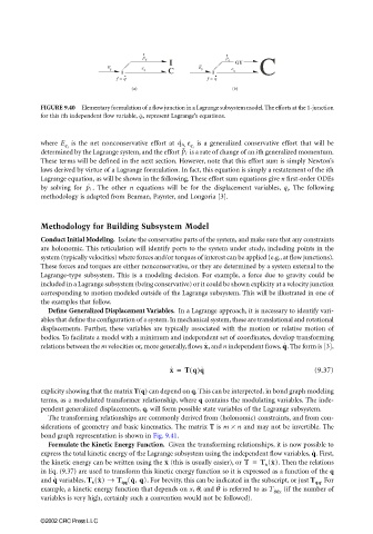
FIGURE 9.40 Elementary formulation of a flow junction in a Lagrange subsystem model. The efforts at the 1-junction
for this ith independent flow variable, , represent Lagrange’s equations.
q ˙ i

, is a generalized conservative effort that will be
where E q i is the net nonconservative effort at q ˙ i e q i
determined by the Lagrange system, and the effort p ˜ ˙ i is a rate of change of an ith generalized momentum.
These terms will be defined in the next section. However, note that this effort sum is simply Newton’s
laws derived by virtue of a Lagrange formulation. In fact, this equation is simply a restatement of the ith
Lagrange equation, as will be shown in the following. These effort sum equations give n first-order ODEs
by solving for p ˙ i . The other n equations will be for the displacement variables, q i . The following
methodology is adapted from Beaman, Paynter, and Longoria [3].

Methodology for Building Subsystem Model
Conduct Initial Modeling. Isolate the conservative parts of the system, and make sure that any constraints
are holonomic. This reticulation will identify ports to the system under study, including points in the
system (typically velocities) where forces and/or torques of interest can be applied (e.g., at flow junctions).
These forces and torques are either nonconservative, or they are determined by a system external to the
Lagrange-type subsystem. This is a modeling decision. For example, a force due to gravity could be
included in a Lagrange subsystem (being conservative) or it could be shown explicity at a velocity junction
corresponding to motion modeled outside of the Lagrange subsystem. This will be illustrated in one of
the examples that follow.
Define Generalized Displacement Variables. In a Lagrange approach, it is necessary to identify vari-
ables that define the configuration of a system. In mechanical system, these are translational and rotational
displacements. Further, these variables are typically associated with the motion or relative motion of
bodies. To facilitate a model with a minimum and independent set of coordinates, develop transforming
q ˙ .
relations between the m velocities or, more generally, flows and n independent flows, The form is [3],
x ˙ ,
x ˙ = Tq()q ˙ (9.37)

explicity showing that the matrix T(q) can depend on q. This can be interpreted, in bond graph modeling
terms, as a modulated transformer relationship, where q contains the modulating variables. The inde-
pendent generalized displacements, q, will form possible state variables of the Lagrange subsystem.
The transforming relationships are commonly derived from (holonomic) constraints, and from con-
siderations of geometry and basic kinematics. The matrix T is m × n and may not be invertible. The
bond graph representation is shown in Fig. 9.41.
Formulate the Kinetic Energy Function. Given the transforming relationships, it is now possible to
q ˙ .
express the total kinetic energy of the Lagrange subsystem using the independent flow variables, First,
the kinetic energy can be written using the (this is usually easier), or T = T ˙ (x ˙). Then the relations
x ˙
x
in Eq. (9.37) are used to transform this kinetic energy function so it is expressed as a function of the q
q ˙
and variables, T ˙ (x ˙) → T ˙ (q ˙ , q). For brevity, this can be indicated in the subscript, or just T ˙ qq . For
x
qq
example, a kinetic energy function that depends on x, θ, and is referred to as θ (if the number of
˙
T ˙
θθx
variables is very high, certainly such a convention would not be followed).
©2002 CRC Press LLC