Page 173 - The Mechatronics Handbook

0066-frame-C09 Page 47 Friday, January 18, 2002 11:01 AM

φ
ω s
ω z,b
ψ z, z a Bearing axis
I:I x
z b
ω
T x
x
φ 1
0 y b
x φ ψ h z G G h y
x a
ψ y a T y T z 1 T L
θ Τ s
x b 1 G 1
y θ All mass assumed ω Load torque
Driving or shaft torque concentrated at rotor. y h x ω z model
(aligned with z) ψ I:I y I:I z
Whirling mode of disk Load torque
is described by θ.
Disk center, C Τ L
ω z
(a) (b)
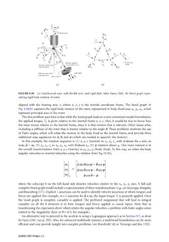
FIGURE 9.38 (a) Cantilevered rotor with flexible joint and rigid shaft (after Vance [36]). (b) Bond graph repre-
senting rigid body rotation of rotor.

aligned with the bearing axis, z, where x, y, z is the inertial coordinate frame. The bond graph in
Fig. 9.38(b) captures the rigid body motion of the rotor, represented in body-fixed axes x b , y b , z b , which
represent principal axes of the rotor.
The first problem seen here is that while the bond graph leads to a very convenient model formulation,
the applied torque, T s , is given relative to the inertial frame x, y, z. Also, it would be nice to know how
the rotor moves relative to the inertial frame, since it is that motion that is relevant. Other issues arise,
including a stiffness of the rotor that is known relative to the angle θ. These problems motivate the use
of Euler angles, which will relate the motion in the body fixed to the inertial frame, and provide three
additional state equations for φ, θ, and ψ (which are needed to quantify the motion).
In this example, the rotation sequence is (1) x, y, z (inertial) to x a , y b , z c , with φ about the z-axis, so
note, = ω s , (2) x a , y a , z a to x b , y b , z b , with θ about x a , (3) ψ rotation about z b . Our main interest is inφ
˙
the overall transformation from x, y, z (inertia) to x b , y b , z b (body-fixed). In this way, we relate the body
angular velocities to inertial velocities using the relation from Eq. (9.20),

˙
˙
φ sin θsin ψ + θcos ψ
ω x
=
˙
˙
–
ω y φ sin θcos ψ θ sin ψ
φ cos
ω z b ˙ θ + ψ ˙
where the subscript b on the left-hand side denotes velocities relative to the x b , y b , z b axes. A full and
complete bond graph would include a representation of these transformations (e.g., see Karnopp, Margolis,
and Rosenberg [17]). Explicit 1-junctions can be used to identify velocity junctions at which torques and
˙
forces are applied. For example, at a 1-junction for = ω z , the input torque T s is properly applied. Onceφ
the bond graph is complete, causality is applied. The preferred assignment that will lead to integral
causality on all the I elements is to have torques and forces applied as causal inputs. Note that in
transforming the expression above which relates the angular velocities, a problem with Euler angles arises
related to the singularity (here at θ = π/2, for example).
An alternative way to proceed in the analysis is using a Lagrangian approach as in Section 9.7, as done
by Vance [36] (see p. 292). Also, for advanced multibody systems, a multibond formulation can be more
efficient and may provide insight into complex problems (see Breedveld [4] or Tiernego and Bos [35]).

©2002 CRC Press LLC