Page 670 - The Mechatronics Handbook

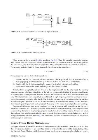
FIGURE 21.8 Complete model in the form of ideal physical elements.

FIGURE 21.9 Model extended with transmission.

When we expand the complete Fig. 21.6 we obtain Fig. 21.8. When this model is processed a message
pops up that indicates that inertia 2 has a dependent state. The two inertias in this model always have
the same speed, and therefore, they are dependent. They cannot have independent initial conditions.
The message indicates that this element can only be written in derivative form:

T = J dω/dt (21.7)
There are several ways to deal with this problem.
1. The two inertias can be combined into one inertia (the program will do this automatically). A
message pops up that the dependency of the two inertias has been solved symbolically.
2. Dealing with the derivative causality by means of an implicit integration algorithm.
3. The transmission can be added, including some flexibility in the belt.
If the flexibility is negligible, solution 1 leads to the simplest model. On the other hand, the warning
raises the question whether the flexibility of the belt can be disregarded indeed. If not, the model has to
be extended with a spring element. It should be noted that this should not be done for numerical reasons
only. If the transmission were very stiff, this would result in high-frequency dynamics and lead to unnec-
essary slow simulations. On the other hand, if the flexibility is important, as it is in this system, the warning
draws the designer’s attention to the fact that the model may be oversimplified. In Fig. 21.9 the transmis-
sion, including a spring element, has been added. Processing of this model does not produce any warnings.
This example illustrates how modern software can help to come up with a model that has the com-
plexity that is needed for a particular problem. Physical models, in the form of an iconic diagram, based
on connecting elements by means of power ports, may help in this modeling process. The user can select
the preferred view, whether this is a bond graph, an iconic diagram with ideal physical element, or a view
using higher lever submodels, like in Fig. 21.6. In the next section it will be shown how to use this model
for the design of controllers.

Control System Design Methodologies

Many processes can be reasonably well controlled by means of PID controllers. This is due to the fact that
these processes can be more or less accurately described by means of a second-order model. Tuning rules,
like those of Ziegler Nichols, enable less experienced people to tune such controllers. Relatively simple

©2002 CRC Press LLC