Page 672 - The Mechatronics Handbook

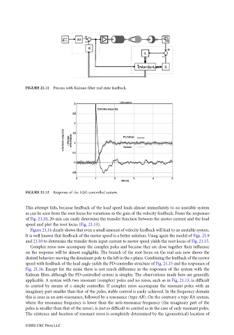
FIGURE 21.11 Process with Kalman filter and state feedback.

FIGURE 21.12 Response of the LQG-controlled system.

This attempt fails, because feedback of the load speed leads almost immediately to an unstable system
as can be seen from the root locus for variations in the gain of the velocity feedback. From the responses
of Fig. 21.10, 20-sim can easily determine the transfer function between the motor current and the load
speed and plot the root locus (Fig. 21.13).
Figure 21.14 clearly shows that even a small amount of velocity feedback will lead to an unstable system.
It is well known that feedback of the motor speed is a better solution. Using again the model of Figs. 21.9
and 21.10 to determine the transfer from input current to motor speed yields the root locus of Fig. 21.15.
Complex zeros now accompany the complex poles and because they are close together their influence
on the response will be almost negligible. The branch of the root locus on the real axis now shows the
desired behavior: moving the dominant pole to the left in the s-plane. Combining the feedback of the motor
speed with feedback of the load angle yields the PD-controller structure of Fig. 21.15 and the responses of
Fig. 21.16. Except for the noise there is not much difference in the responses of the system with the
Kalman filter, although the PD-controlled system is simpler. The observations made here are generally
applicable. A system with two resonant (complex) poles and no zeros, such as in Fig. 21.13, is difficult
to control by means of a simple controller. If complex zeros accompany the resonant poles with an
imaginary part smaller than that of the poles, stable control is easily achieved. In the frequency domain
this is seen as an anti-resonance, followed by a resonance (type AR). On the contrary a type RA system,
where the resonance frequency is lower than the anti-resonance frequency (the imaginary part of the
poles is smaller than that of the zeros), is just as difficult to control as in the case of only resonant poles.
The existence and location of resonant zeros is completely determined by the (geometrical) location of

©2002 CRC Press LLC