Page 901 - The Mechatronics Handbook

0066_Frame_C30 Page 12 Thursday, January 10, 2002 4:43 PM

We will show how this optimal control problem—and problems like it—can be readily solved using
computer-aided design soflware (e.g., MATLAB, robust control toolbox, m-tools).

Comment 30.9 (Construction of Generalized Plant G)
Generalized plants G are very easy to construct within SIMULINK. Input port blocks may be used to
specify exogenous signals w and controls u. Output port blocks may be used to specify regulated signals
z and measurements y. The “linmod” command may be applied to the constructed block diagram
(SIMULINK file) to obtain a two-port state space (A, B = [B 1 B 2 ], C = [C 1 ; C 2 ], D = [D 11 D 12 ; D 21 D 22 ])
representation for G. The syntax for the command is as follows:

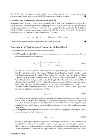
[ a, b, c, d ] = linmod (‘filename’)

This method enables one to create generalized plant models quickly.

2
Overview of HH Optimization Problems to Be Considered
Three fundamental problems are considered in this chapter:
1. HH 2 Output Feedback Problem. The solution to this problem is an optimal model-based dynamic
compensator possessing the structure

AB 2 G c – H f C 2 H f
–
K opt = (30.61)
– G c O n ×n
u
where G c , is a control gain (state feedback) matrix and H f is a filter gain (observer) matrix. G c is
found by using the solution of a Control Algebraic Riccati Equation (CARE)—similar to that
found in Linear Quadratic Regulator (LQR) problems. H f is found by using the solution of a Filter
Algebraic Riccati Equation (FARE)—similar to that found in Kalman–Bucy Filtering (KBF) prob-
lems. The structure of K opt , G c , and H f can be thought of as the solution to a classical Linear
Quadratic Gaussian (LQG) control problem which gives rise to the well known separation prin-
ciple: closed loop poles are the eigenvalues of A − B 2 G c , and the eigenvalues of A − H f C 2 .
2. HH 2 State Feedback Problem. The solution to this problem is an optimal constant gain (state
feedback) compensator possessing the structure

K opt = – G c (30.62)

where G c is a control gain (state feedback) matrix found by using the solution to a CARE—similar
to that found in LQR problems. The poles of the resulting closed loop system are the eigenvalues
of A− B 2 G c . In short, this problem should be viewed as a mechanism for computing control gain
matrices G c that may be used in a state feedback application or in a model-based compensator
application.
3. HH 2 Output Injection Problem. The solution to this problem is an optimal constant gain (static)
compensator possessing the structure

K opt = – H f (30.63)

where H f is a filter gain (observer) matrix found by using the solution to a FARE—similar to that
found in KBF problems. The poles of the resulting closed loop system are the eigenvalues of A −
H f C 2 . In short, this problem should be viewed as a mechanism for computing filter gain matrices
H f that may be used in a state estimation application or in a model-based compensator application.

©2002 CRC Press LLC