Page 902 - The Mechatronics Handbook

0066_Frame_C30 Page 13 Thursday, January 10, 2002 4:43 PM

30.3 HH 2 Output Feedback Problem

2
In this section, we consider the H output feedback problem. This problem results in model-based
(dynamic) compensators involving a control gain (state feedback) matrix G c and a filter gain (observer)
matrix H f . As such, the problem generalizes the ideas presented in classical LQG theory.
2
The following “standard” H output feedback problem assumption is now made.
Assumption 30.1 (HH 2 Output Feedback Problem)
Throughout this section, it will be assumed that
1. Plant G 22 Assumption. (A, B 2 , C 2 ) stabilizable and detectable.
• This assumption is necessary and suficient for the existance of a proper internally stabilizing
controller K. With this assumption, the following model based (observer based) controller
stabilizes the feedback loop in Fig. 30.1:

(
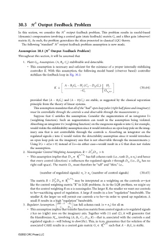
AB 2 G c – H f C 2 – D 22 G c ) H f
–
K = (30.64)
– G c O n ×n
u
provided that (A − B 2 G c ) and (A − H f C 2 ) are stable, as suggested by the classical separation
principle from the theory of linear systems.
This assumption mandates that all of the “bad” open loop poles (right half plane and imaginary)
must be controllable through the controls u and observable through the measurements y.
Suppose that G satisfies the assumption. Consider the augmentation of an integrator I/s
(weighting function). Such an augmentation can result in the assumption being violated.
Absorbing an integrator I/s (weighting function) on the exogenous signals w into G, for example,
would violate the stabilizability assumption since it would introduce an open loop pole on the imag-
inary axis that is not controllable through the controls u. Absorbing an integrator on the
regulated signals z into G would violate the detectability assumption since it would introduce
an open loop pole on the imaginary axis that is not observable through the measurements y.
Using I/(s + )( > 0) instead of I/s––in either case—would result in a G that does not violate
the assumption.
T
2. Nonsingular Control Weighting Assumption. R = D 12 D 12 > 0.
n ×
n
• This assumption implies that D 12 ∈ R z u has full column rank (i.e., rank D 12 = n u ) and hence
that every control (direction) u influences the regulated signals z through D 12 (i.e., D 12 has no
right null space). The matrix D 12 must therefore be “tall” and “thin;” i.e.,

(number of regulated signals) n ≥ n (number of control signals) (30.65)
z
u
n × n
T
The matrix R = D 21 D 12 ∈ R u u may be interpreted as a weighting on the controls u—just
like the control weighting matrix “R” in LQR problems. As in the LQR problem, we might say
that the control weighting R on u is nonsingular. The larger R, the smaller we want our controls
to be—sacrificing speed of regulation. A large R results in a low “regulation” bandwidth. The
smaller R, the larger we will permit our controls u to be—in order to speed up regulation. A
small R results in a high “regulation” bandwidth.
–
jwIA – B 2
3. Regulator Assumption. has full column rank (n + n u ) for all w.
C 1 D 12
• This assumption implies that transfer function matrix from control signals u to regulated signals
z has no (right) zero on the imaginary axis. Together with (1) and (2), it will guarantee that
the Hamiltonian H con involving (A, B 2 , C 1 , D 12 , R)—that is, associated with the controls u and
regulated signals z—will belong to dom(Ric). This, in turn, guarantees that the solution of the
associated CARE results in a control gain matrix G c ∈ R n ×n such that A − B 2 G c is stable.
u

©2002 CRC Press LLC