Page 906 - The Mechatronics Handbook

0066_Frame_C30 Page 17 Thursday, January 10, 2002 4:43 PM

2
2
The same is true for H output feedback designs. We will show how the H framework presented can
be manipulated to solve LQG/LTR problems which yield model-based controllers with desirable stability
robustness margins—comparable to those found in feedback designs resulting from suitably formulated
LQR and KBF problems (e.g., infinite upward gain margin, at least 6 dB downward gain margin, at least
±60° phase margin).
2
The following example shows how weighted H mixed sensitivity optimization may be used to design
a controller for an unstable system with a time delay.

Example 30.2 (Weighted HH 2 Mixed Sensitivity Design
for Unstable System with Time Delay)
In this example, we consider an unstable system with a time delay ∆ = 0.05 s (50 ms). The system is
modeled (approximately) as follows:

–
1
40 s
2/∆ s
1
–
P ≈ ---------- ----------------- = ---------- -------------- (30.87)
s 1 2/∆ + s s 1 40 + s
–
–
Design Specifications. The objective is to design a controller K that satisfies the following closed loop
specifications: (1) closed loop stability, (2) sensitivity below −60 dB for all frequencies below 0.1 rad/s,
(3) sensitivity gain crossover between 2 and 3 rad/s, (4) peak sensitivity below 5 dB, (5) peak comple-
mentary sensitivity below 10 dB.
2
Weighted H Mixed Sensitivity Problem. To achieve the above specifications, we formulated a weighted
2
H mixed sensitivity problem—with a weighting W 1 on the sensitivity S and a weighting W 2 on KS; i.e.,
W 1 S
2 = min (30.88)
min T wz
K H K W 2 KS H 2
The weighting functions used were as follows:
10
k 1
W 1 = ------------- = ------------------ (30.89)
s + p 1 s + 0.01
(
(
k 2 s + z 2 ) 0.1 s + 40)
W 2 = ---------------------- = -------------------------- (30.90)
s + p 2 s + 2
W I penalizes the sensitivity S heavily at low frequencies (e.g., below 0.001 rad/s). Above 0.1 rad/s, W I is
small and W 2 penalizes KS (with magnitude greater than unity) until about 4 rad/s. Since the solution
2
of our H optimization depends in a very complex manner on the parameters that define W I and W 2 , it
should be no surprise that it took a while to determine suitable parameters.
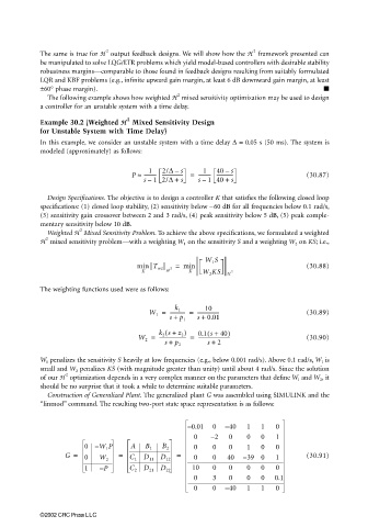
Construction of Generalized Plant. The generalized plant G was assembled using SIMULINK and the
“linmod” command. The resulting two-port state space representation is as follows:

– 0.01 0 – 40 1 1 0
0 – 2 0 0 0 1
0 – W 1 P A B 1 B 2 0 0 0 1 0 0
G = 0 W 2 = C 1 D 11 D 12 = 0 0 40 – 39 0 1 (30.91)

1 – P C 2 D 21 D 22 10 0 0 0 0 0
0 3 0 0 0 0.1
0 0 – 40 1 1 0

©2002 CRC Press LLC