Page 911 - The Mechatronics Handbook

0066_Frame_C30 Page 22 Thursday, January 10, 2002 4:44 PM

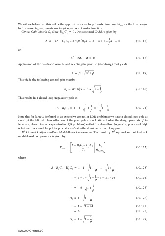
We will see below that this will be the approximate open loop transfer function PK opt for the final design.
In this sense, G KF represents our target open loop transfer function.
Control Gain Matrix G c . Since D 12 C 1 = 0 , the associated CARE is given by
T
A X + XA + C 1 C 1 – XB 2 R B 2 X = X + X + 1 – 1 2 0 (30.117)
---X =
T
T
1
–
r
or
2
X – 2rX r = 0 (30.118)
–
Application of the quadratic formula and selecting the positive (stabilizing) root yields:
2
X = r + r + r (30.119)
This yields the following control gain matrix:

G c = R B 2 X = 1 + 1 + 1 (30.120)
−1
T
---
r
This results in a closed loop (regulator) pole at
--- =
AB 2 G c = 11 – 1 + 1 – 1 + 1 (30.121)
---
–
–
r r
Note that for large r (referred to as expensive control in LQR problems) we have a closed loop pole at
s = −1, at the left half plane reflection of the plant pole at s = 1. We will select the design parameter r to
be small (referred to as cheap control in LQR problems) so that this closed loop (regulator) pole s ≈ −1/ r
is fast and the closed loop filter pole at s = −5 at is the dominant closed loop pole.
2
2
H Optimal Output Feedback Model-Based Compensator. The resulting H optimal output feedback
model-based compensator is given by
AB 2 G c – H f C 2 H f
–
K opt = (30.122)
– G c 0 n × n
u y
where

1
1
1
–
–
AB 2 G c – H f C 2 = 11 – 1 + --- – – 1 + --- (30.123)
r m
= 11 – 1 + 1 1 1 + 24 (30.124)
--- – –
–
r
1
= – 6 – 1 + --- (30.125)
r
1
H f = 1 + 1 + --- (30.126)
m
= 1 + 1 + 24 (30.127)
= 6 (30.128)
G c = 1 + 1 + 1 (30.129)
---
r

©2002 CRC Press LLC