Page 915 - The Mechatronics Handbook

0066_Frame_C30 Page 26 Thursday, January 10, 2002 4:44 PM

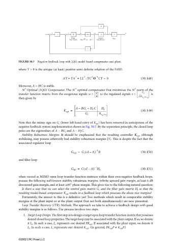
FIGURE 30.7 Negative feedback loop with LQG model-based compensator and plant.
where Y > 0 is the unique (at least) positive semi-definite solution of the FARE:

AY + YA + LL – YC Θ CY = 0 (30.148)
T
−1
T
T
Moreover, A − HC is stable.
2
2
2
H Optimal (LQG) Compensator. The H optimal compensator that minimizes the H norm of the
transfer function matrix from the exogenous signals w = x to the regulated signals z = C x is
q rI n u ×
then given by n u
–
ABG c – H f C H f
K opt = (30.149)
G c 0 n × n
u
Note that the minus sign on G c (lower left hand entry of K opt ) has been removed in anticipation of the
negative feedback system implementation shown in Fig. 30.7. By the separation principle, the closed loop
poles are the eigenvalues of A − BG c and A − H f C.
Stability Robustness Margins. It should be emphasized that the resulting controller K opt , although
stabilizing, may possess arbitrarily bad stability robustness margins [3]. This is despite the fact that the
associated regulator loop

G LQ = G c sI A) B (30.150)
(
−1
–
and filter loop

(
G KF = CsI A) H f (30.151)
−1
–
when viewed as MIMO open loop transfer function matrices within their own negative feedback loops,
possess the following well-known stability robustness margins: infinite upward gain margin, at least 6 dB
downward gain margin, and at least ±60° phase margin. This gives rise to the following natural question:
Is there a way that we can select the control gain matrix G c and the filter gain matrix H f so that the
resulting model-based compensator K opt results in a feedback loop which possesses the above nice margins?
Fortunately, the answer to this is a definitive yes! Two methods which result in comparable stability
margins at the plant input or at the plant output (but not both simultaneously) are now presented.
Loop Transfer Recovery (LTR) Methods. The approach we take to achieve a feedback design with good
stability margins is as follows. The process involves two steps.
1. Target Loop Design. The first step is to design a target open loop transfer function matrix that possesses
desired closed loop properties. The target loop may be associated with the plant output. If so, we denote
it L o . In such a case, L o represents our desired PK opt . If associated with the plant input, we denote it
L i . In such a case, L i represents our desired K opt . (In general, PK opt P ≠ K opt P.)

©2002 CRC Press LLC