Page 916 - The Mechatronics Handbook

0066_Frame_C30 Page 27 Thursday, January 10, 2002 4:44 PM

2. Target Loop Recovery Via Model-Based Compensator. The second step is to use a model-based com-
pensator K opt = [A − BG c − H f C, H, G] to recover the target loop (either L o or L i ).
If we want to recover L o (i.e., good properties at that plant output), then we want PK opt ≈ L o .
This is called loop transfer recovery at the plant output (LTRO).
If we want to recover L i (i.e., good properties at that plant input), then we want K opt P ≈ L i ,.
This is called loop transfer recovery at the plant input (LTRI).
Note: In general, the properties associated with breaking the loop at the plant output (properties
of PK opt ) are different (perhaps very different) from those associated with breaking the loop at the
plant input (properties of K opt P). It is usually very difficult for PK opt and K opt P to both possess
great properties (e.g., margins, etc.). Typically, a designer must trade off nice properties at the
plant output for nice properties at the plant input, or vice versa.
2
H -based methods for LTRO and LTRI are now presented.
• Loop Transfer Recovery at Plant Output (LTRO).
−l
1. Design of Target Loop L o . The first step is to design a target loop L o = C(sI − A) H f with desirable
closed loop properties (e.g., stability, sensitivity, complementary sensitivity, stability robustness
margins, etc). This may be done using any method! (Any method you feel comfortable enough
with.)
One procedure that results in good properties at the plant output is based on KBF methods.
−l
The idea is to select the design (shaping) matrix L so that the singular values G FOL = C(sI − A) L
look nice; e.g., large minimum singular value at low frequencies, small maximum singular
value at high frequencies, singular values cross 0 dB with slopes of −20 dB/dec, etc.
—using m > 0 to adjust the bandwidth of
We then solve the FARE with A, L, C, Θ = mI n ×n
y y
−l
our target loop L o = G KF = C(sI − A) H f . A smaller (larger) m results in a larger (smaller)
bandwidth.
Guidelines for Shaping of Target Loop L o = G KF .
• The so-called Kalman Frequency Domain Equality (KFDE) guides our loop shaping:
1
1
[
(
(
(
[ I + G KF jw)] I + G KF jw)] H = I + -------G FOL jw( ) -------G FOL jw) H (30.152)
m m
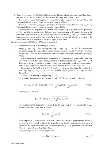
From this, it follows that
1
(
[
s i I + G KF jw)] = 1 + ---s i G FOL jw([ )] (30.153)
2
m
This suggests that by shaping G FOL , we can shape the target loop L o = G KF . Specifically, if G FOL
is large at low frequencies, then we expect
1
(
G KF jw) ≈ -------G FOL jw( ) (30.154)
m
at low frequencies. This shows that the matrix L should be used for shaping the target loop L o =
G KF while m > 0 is used to adjust the target loop bandwidth—decreasing/increasing m to
raise/lower the target loop bandwidth. The resulting loop L o = G KF is guaranteed to possess nice
closed loop properties as described below.
• The above singular value relation implies that

(
[
s min I + G KF jw)] ≥ 1 (30.155)

©2002 CRC Press LLC