Page 922 - The Mechatronics Handbook

0066_Frame_C30 Page 33 Thursday, January 10, 2002 4:44 PM

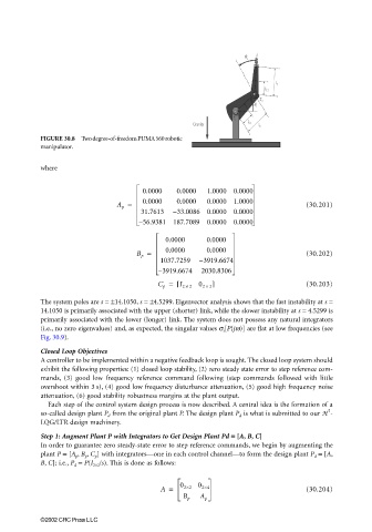
FIGURE 30.8 Two degree-of-freedom PUMA 560 robotic
manipulator.

where

0.0000 0.0000 1.0000 0.0000
A p = 0.0000 0.0000 0.0000 1.0000 (30.201)
31.7613 – 33.0086 0.0000 0.0000
– 56.9381 187.7089 0.0000 0.0000

0.0000 0.0000
0.0000 0.0000
B p = (30.202)
1037.7259 – 3919.6674
– 3919.6674 2030.8306
C p = [ I 2 × 2 0 2 × ] (30.203)
2
The system poles are s = ±14.1050, s = ±4.5299. Eigenvector analysis shows that the fast instability at s =
14.1050 is primarily associated with the upper (shorter) link, while the slower instability at s = 4.5299 is
primarily associated with the lower (longer) link. The system does not possess any natural integrators
(i.e., no zero eigenvalues) and, as expected, the singular values σ i [P(jω)] are flat at low frequencies (see
Fig. 30.9).
Closed Loop Objectives
A controller to be implemented within a negative feedback loop is sought. The closed loop system should
exhibit the following properties: (1) closed loop stability, (2) zero steady state error to step reference com-
mands, (3) good low frequency reference command following (step commands followed with little
overshoot within 3 s), (4) good low frequency disturbance attenuation, (5) good high frequency noise
attenuation, (6) good stability robustness margins at the plant output.
Each step of the control system design process is now described. A central idea is the formation of a
2
so-called design plant P d from the original plant P. The design plant P d is what is submitted to our H -
LQG/LTR design machinery.
Step 1: Augment Plant P with Integrators to Get Design Plant Pd == == [A, B, C]
In order to guarantee zero steady-state error to step reference commands, we begin by augmenting the
plant P = [A p , B p , C p ] with integrators—one in each control channel—to form the design plant P d = [A,
B, C]; i.e., P d = P(I 2×2 /s). This is done as follows:

A = 0 2×2 0 2×4 (30.204)
B p A p

©2002 CRC Press LLC