Page 923 - The Mechatronics Handbook

0066_Frame_C30 Page 34 Thursday, January 10, 2002 4:44 PM

Outputs: θ , θ (deg); Inputs: τ , τ (lb–ft)
1 2 1 2
30
20
10

0
Singular Values (dB) −10

−20

−30

−40

−50

−60
−1 0 1 2
10 10 10 10
Frequency (rad/sec)
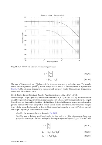
FIGURE 30.9 PUMA 560 robotic manipulator singular values.

B = 1 2×2 (30.205)
0 4×2
C = [ 0 2×2 C p ] (30.206)

The state of this system is x = x i where x i is the integrator state and x p is the plant state. The singular
x p
values for the augmented system P d exhibit a slope of −20 dB/dec at low frequencies as expected (see
Fig. 30.10). The minimum singular value crosses zero dB just above 1 rad/s. The maximum singular value
crosses zero dB at about 8 rad/s.
−− − −l
Step 2: Design Target Open Loop Transfer Function Matrix L o == == G KF == == C(sI −− −− A) H f
−l
Next we design a target open loop transfer function matrix L o = G KF = C(sI − A) H f that has desirable
closed loop properties (e.g., sensitivity singular values, pole locations, stability margins, etc.) at the output.
To do this, we use Kalman Filtering ideas. Like LQR loops designed without a cross-state-control-coupling
penalty, Kalman Filter loops designed in similar fashion exhibit desirable stability robustness margins
(e.g., infinite upward gain margin, at least 6 dB downward gain margin, at least ±60° phase margin).
This target loop design is carried out as follows:
• Consider the augmented system shown in Fig. 30.11.
It will be used to design a target loop transfer function matrix L o = G KF with desirable closed loop
−l
properties at the output. To do so, we begin by forming an augmented system G FOL = C(sI − A) L with

L = L L (30.207)

L H
(
L L = [ C p – A p ) B p ] – 1 (30.208)
–
1
L H = – ( A p ) B p L L (30.209)
–
1
©2002 CRC Press LLC