Page 925 - The Mechatronics Handbook

0066_Frame_C30 Page 36 Thursday, January 10, 2002 4:44 PM

G Singular Values
FOL
30
20

10
Singular Values (dB) −10 0

−20

−30

−40
10 −1 10 0 10 1 10 2
Frequency (rad/sec)
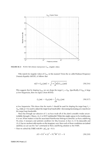
FIGURE 30.12 PUMA 560 robotic manipulator G FOL singular values.

Why match the singular values of G FOL in this manner? From the so-called Kalman Frequency
Domain Equality (KFDE), it follows that

[
s i I + G KF jw)] = 1 + 1 2 )] (30.216)
---s i G FOL jw([
(
m
This suggests that by shaping G FOL , we can shape the target L o = G KF . Specifically, if G FOL is large
at low frequencies, then we expect (from KFDE)

1
(
L o jw) = G KF jw) ≈ -------G FOL jw( ) (30.217)
(
m
at low frequencies. This shows that the matrix L should be used for shaping the target loop L o =
G KF while µ > 0 is used to adjust the target loop bandwidth—decreasing/increasing m to raise/lower
the target loop bandwidth.
Note that through our selection of L, we have made all of the plant’s unstable modes uncon-
trollable through L. Hence, (A, L) is NOT stabilizable! While this might appear to be troublesome,
it is not. What matters is that the associated Hamiltonian belongs to dom(Ric) so that a stabilizing
H f exists. A necessary and suficient condition for this, however, is that (A, C) be detectable and
(A, L) has no unobservable modes on the imaginary axis. Since each of these conditions are indeed
satisfied, we can use the “are” command to find a stabilizing solution to the FARE.
• Next we solved the FARE with Θ = µI 2×2 (m = 0.1):

–
1
AY + YA + LL – YC Θ CY = 0 (30.218)
T
T
T
©2002 CRC Press LLC