Page 929 - The Mechatronics Handbook

0066_Frame_C30 Page 40 Thursday, January 10, 2002 4:44 PM

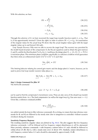
With this selection, we have

PK = P----- (30.232)
K d
s
I 2 ×
= P---------K d (30.233)
2
s
= P d K d (30.234)
≈ L o = G KF (30.235)

Through this selection of K, we have recovered the target loop transfer function matrix L o = G KF . That
is, K has approximately inverted P (from the right) in order to achieve PK ≈ L o = G KF . An examination
of the singular values for the actual loop PK shows that the actual singular values agree with the target
singular values up to and beyond 100 rad/s.
Loop Transfer Recovery. Why were we able to recover the target loop? The recovery was permitted by
the model-based structure of the compensator K, the Riccati equations used to obtain the gain matrices
G c and H f , and the fact that the plant P = [A p , B p , C p ] (and hence the design plant P d = [A, B, C] = P(I/s)
is minimum phase. The minimum phase condition, specifically, is a suficient condition which guarantees
T
T
that there exists an orthonormal matrix U(U U = UU = I) such that
lim rG c = UC (30.236)
r → 0 +

This limiting behavior relating the control gain matrix and the design plant’s C matrix, however, can be
used to prove that loop transfer recovery takes place; i.e.,

lim P d K d = lim PK = L o = G KF (30.237)
r→ 0 + r → 0 +

Step 5: Design Command Pre-filter W
The MATLAB command

t 0 ab ∗ –( gh ∗ c, h, g) (30.238)
–

can be used to find the compensator’s transmission zeros. These are also zeros of the closed loop transfer
function matrix from r to y. The final compensator (as well as the target loop G KF ) has zeros near s ≈ −1.2.
Given this, a reference command prefilter

1.2
W = ----------------I 2 × (30.239)
s + 1.2 2

was added outside the loop to filter reference commands. By so doing, we ensure that step reference com-
mands for θ 1 and θ 2 are followed in the steady state (due to integrators in controller) without excessive
overshoot during the transient.
Sensitivity Frequency Response
The resulting sensitivity singular values are plotted in Fig. 30.16. The plot suggests that low frequency
reference commands r will be followed and low frequency output disturbances d o will be attenuated.
More precisely, reference commands r with frequency content below 0.3 rad/s should be followed to
within about 20 dB; that is, with a steady-state error of about 10%. Similarly, output disturbances d o
with frequency content below 0.3 rad/s should be attenuated by approximately 20 dB.

©2002 CRC Press LLC