Page 200 - Thomson, William Tyrrell-Theory of Vibration with Applications-Taylor _ Francis (2010)

Sec. 6.7 Modal Matrix P 187

6.7 MODAL MATRIX P

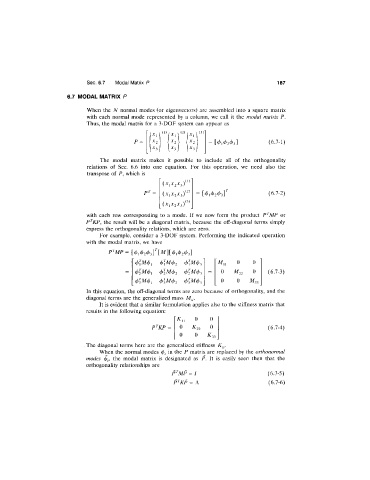
When the N normal modes (or eigenvectors) are assembled into a square matrix
with each normal mode represented by a column, we call it the modal matrix P.
Thus, the modal matrix for a 3-DOF system can appear as
(2) / (3)
^'1 /■ V ,) 1 -^1
(6.7-1)
^3 I 1 U 3 1
The modal matrix makes it possible to include all of the orthogonality
relations of Sec. 6.6 into one equation. For this operation, we need also the
transpose of P, which is
(1)
(X^X2X^)
(2)
(X^X2X2) = [(/>i(/>2(/)3]^ (6.7-2)
(X1X2X3) (3)

with each row corresponding to a mode. If we now form the product P^MP or
P^KP, the result will be a diagonal matrix, because the off-diagonal terms simply
express the orthogonality relations, which are zero.
For example, consider a 3-DOF system. Performing the indicated operation
with the modal matrix, we have

4>]M4>2 0 0
4>Im 4>2 4,lM4>2 = 0 M22 0 (6.7-3)
V,M4>2 0 0
In this equation, the off-diagonal terms are zero because of orthogonality, and the
diagonal terms are the generalized mass
It is evident that a similar formulation applies also to the stiffness matrix that
results in the following equation:
Ku 0 0
P^fiP = 0 K22 0 (6.7-4)
0 0 K, 33

The diagonal terms here are the generalized stiffness K-.
,
When the normal modes (/> in the P matrix are replaced by the orthonormal
modes (/>,, the modal matrix is designated as P. It is easily seen then that the
orthogonality relationships are
P^MP = / (6.7-5)
P^K P = A (6.7-6)