Page 25 - Thomson, William Tyrrell-Theory of Vibration with Applications-Taylor _ Francis (2010)

Oscillatory Motion Chap. 1
12

0.4 h
0.3
0.2
0.1
, ^ r - r r " r -
0 1 2 3 4 5 6 7 8 9 lO II I2

90® y
y
y
y
______________
y
y
y
y
-90®
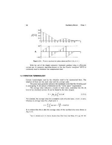
Figure 1.2-2. Fourier spectrum for pulses shown in Prob. 1-16, k = \.
With the aid of the digital computer, harmonic analysis today is efficiently
carried out. A computer algorithm known as the fast Fourier transform^ (FFT) is
commonly used to minimize the computation time.

1.3 VIBRATION TERMINOLOGY

Certain terminologies used in the vibration need to be represented here. The
simplest of these are the peak value and the average value.
The peak value generally indicates the maximum stress that the vibrating part
is undergoing. It also places a limitation on the “rattle space” requirement.
The average value indicates a steady or static value, somewhat like the dc
level of an electrical current. It can be found by the time integral
1 T ' '
X = lim \ x{t) dt (1.3-1)
T-^oo ^
For example, the average value for a complete cycle of a sine wave, A sin t, is zero;
whereas its average value for a half-cycle is
2A
X = — f ûrvtdt = = 0.637^
77^0 77
It is evident that this is also the average value of the rectified sine wave shown in
Fig. 1.3-1.
^See J. S. Bendat and A. G. Piersol, Random Data (New York: John Wiley, 1971), pp. 305-306.