Page 439 - Thomson, William Tyrrell-Theory of Vibration with Applications-Taylor _ Francis (2010)

426 Random Vibrations Chap. 13

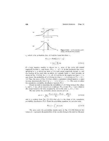
Figure 13.4-2. (a) Cumulative prob­
ability, (b) Probability density.
jfj, which is the probability that x{t) will be found less than Xj.

P ( a i) = P ro b [x (i) <Xj]
'
= lim y XI (13.4-1)
i->00 I
If a large negative number is chosen for Xj, none of the curve will extend
negatively beyond Xj, and, hence, P(x, -oo) = 0. As the horizontal line corre-
sponding to x, is moved up, more of x{t) will extend negatively beyond x,, and
the fraction of the total time in which x{t) extends below Xj must increase, as
shown in Fig. 13.4-2(a). As x oo, all x{t) will lie in the region less than x = oo,
and, hence, the probability of x{t) being less than x = oo is certain, or P{x = qo) =
1.0. Thus, the curve of Fig. 13.4-2(a), which is cumulative toward positive x, must
increase monotonically from 0 at x = -oo to 1.0 at x = -f-oo. The curve is called
the cumulative probability distribution function P{x).
If next we wish to determine the probability of x{t) lying between the values
Xj and X| + Ax, all we need to do is subtract F(xj) from P{x^ -h Ax), which is
also proportional to the time occupied by x{t) in the zone Xj to Xj + Ax.
We now define the probability density function p{x) as

P{x + Ax) —P{x) _ dP(x)

p{x) = lim (13.4-2)
Ax dx
and it is evident from Fig. 13.4-2(b) that p(x) is the slope of the cumulative
probability distribution P{x). From the preceding equation, we can also write
J
(13.4-3)
^ _ rv-
The area under the probability density curve of Fig. 13.4-2(b) between two
values of x represents the probability of the variable being in this interval. Because