Page 438 - Thomson, William Tyrrell-Theory of Vibration with Applications-Taylor _ Francis (2010)

Sec. 13.4 Probability Distribution 425

0> m
n
c C
o
5 I 0.5 I I.0 I.5
0
.
<o/w„
o ^
O' Q.
o) ir
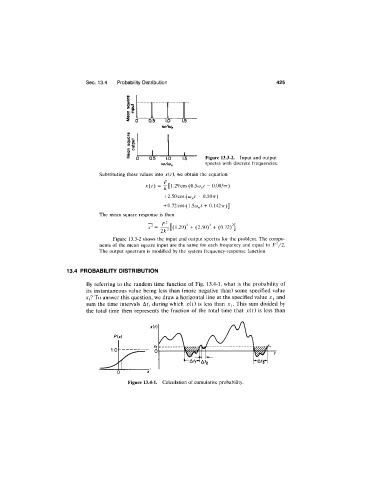
0.5 I.O I.5 Figure 13.3-2. Input and output
w/u>„ spectra with discrete frequencies.

Substituting these values into x{t), we obtain the equation
x(t) = J [1.29cos (0.5o)„i - 0.083tt)
+ 2.50 COS - 0.507t)
+ 0.72 cos (1.5io„r + 0.1427t)]
The mean square response is then
-
X = — I[(1.29f + (2.50)^ + (0.72)‘]
2k^ '
Figure 13.3-2 shows the input and output spectra for the problem. The compo­
nents of the mean square input are the same for each frequency and equal to F^/2.
The output spectrum is modified by the system frequency-response function.

13.4 PROBABILITY DISTRIBUTION
By referring to the random time function of Fig. 13.4-1, what is the probability of
its instantaneous value being less than (more negative than) some specified value
Xj? To answer this question, we draw a horizontal line at the specified value and
sum the time intervals Af- during which x(t) is less than Xj. This sum divided by
the total time then represents the fraction of the total time that x(t) is less than

Figure 13.4-1. Calculation of cumulative probability.