Page 477 - Bird R.B. Transport phenomena

§15.2 The Macroscopic Mechanical Energy Balance 457

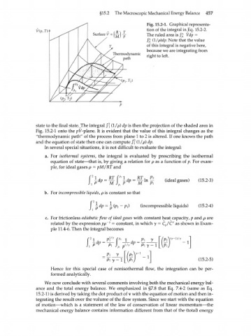
Fig. 15.2=1. Graphical representa-
tion of the integral inEq. 15.2-2.
Surface V = (A) X The ruled area is /£ Wp =
/g; (1 /pWp. Note that the value
of this integral is negative here,
because we are integrating from
Thermodynamic right to left.
path

state to the final state.^The integral /? (1 /p) dp is then the projection of the shaded area in
Fig. 15.2-1 onto the pV-p\ane. It is evident that the value of this integral changes as the
"thermodynamic path" of the process from plane 1 to 2 is altered. If one knows the path
and the equation of state then one can compute /? (1 /p) dp.
In several special situations, it is not difficult to evaluate the integral:
a. For isothermal systems, the integral is evaluated by prescribing the isothermal
equation of state—that is, by giving a relation for p as a function of p. For exam-
ple, for ideal gases p = pM/RT and

l
1

b o For incompressible liquids, p is constant so that

(incompressible liquids) (15.2-4)
с For frictionless adiabatic flow of ideal gases with constant heat capacity, p and p are
y
v
related by the expression pp~ = constant, in which у = C /C as shown in Exam-
p
ple 11.4-6. Then the integral becomes

V\ У 7-1
(15.2-5)

Hence for this special case of nonisothermal flow, the integration can be per-
formed analytically.
We now conclude with several comments involving both the mechanical energy bal-
ance and the total energy balance. We emphasized in §7.8 that Eq. 7.4-2 (same as Eq.
15.2-1) is derived by taking the dot product of v with the equation of motion and then in-
tegrating the result over the volume of the flow system. Since we start with the equation
of motion—which is a statement of the law of conservation of linear momentum—the
mechanical energy balance contains information different from that of the (total) energy